Can Impermanent Loss Be Hedged? A Simulation Study on GammaSwap

A structural explanation of impermanent loss and gain; and a detailed simulation of volatility-based hedging on GammaSwap.

Apr 03, 2026

If you found this useful, the full breakdown with math and simulation is on Substack → [mirador.finance] More deep-dives incoming.

Join our Telegram to get notified first → [https://t.me/Miradortelegram]

INTRODUCTION

Impermanent loss is an inherent risk for liquidity providers (LPs) in Automated Market Makers (AMM) pools. However, GammaSwap, the first on-chain perpetual (perp) options decentralized exchange (DEX), seeks to convert this risk into “Impermanent Gain” by allowing traders to bet on the tokens’ volatility via liquidity loan from AMMs.

How can GammaSwap turn the impermanent loss (IL) to impermanent gain (IG)?

Is hedging IL strategy on GammaSwap really financially viable?

This article is mainly to examine these two questions by deeply diving into its sophisticated mathematical formulas and simulating the hedging strategy’s profitability on GammaSwap.

KEY TAKEAWAYS

In this article, we will clearly examine the effectiveness of hedging IL strategy on GammaSwap via 3 main following sections:

Section 1: Understanding about Impermanent Loss – the problem that LPs mostly concerns when providing liquidity into traditional AMMs like Uniswap V2
Section 2: Explore how GammaSwap turns impermanent loss into impermanent gain and the essence of hedging strategy
Section 3: Examine the viability of GammaSwap’s hedge strategy via realistic numbers

SECTION 1: THE PROBLEM - IMPERMANENT LOSS IN TRADITIONAL AMMS

1/ What Is Impermanent Loss?

For many people, providing liquidity in an AMM pool sounds like a safe strategy in the DeFi game because you don’t need to bet on price direction while still earning trading fees from swappers.

However, one strange-but-inevitable thing happens: even when the asset goes up and you make money, you still earn less than if you had done nothing and just held.

This hidden gap is called “Impermanent loss”.

So, theoretically:

Impermanent loss (IL) is the difference (loss) between providing liquidity (LP) to the AMM compared to simply holding (HODL) those tokens.

It’s called impermanent loss because your loss can be offset or recovered when the token price returns to its initial price, and not a complete loss of money. In practice, IL represents the opportunity cost of LP, trading off the risk of price volatility for the profit from fees.

IL happens only when the token’s price in the AMM pool changes from the time of the initial deposit. It means:

In case of no price change, no IL will occur and LPs will earn a positive profit from the trading fees.
In case of price change, if the trading fee cannot cover IL, the profit of LPs may turn negative, and vice versa.

IL is not caused by a bug, hack, volatility crashes or any bad executions but integrated directly into the algorithms of AMM because of its automatic rebalance mechanism, where the pool’s LPs are forced to sell their assets that are increasing in value and buy those decreasing in value, while token holders are not.

The most familiar spot where IL often occurs is on Constant Product Market Maker (CPMM) pools like Uniswap V2, where the most basic invariant is applied:

$x \cdot y = k$

X: the number of token A (i.e. $ETH)
Y: the number of token B (i.e. $USDC)
K: constant number

When ETH increases, the traders outside will buy ETH (swap USDC for ETH) from the pool as they see an arbitrage opportunity to sell it elsewhere for a profit. It means the AMM pool will automatically sell the increasing ETH, decreasing the quantity of ETH and increasing that of USDC, while their value is equal. And vice versa, when ETH decreases, the pool will buy more ETH. These arbitrage trades are exactly how the AMM continuously rebalances the pool, without the need for an order book or any intermediary.

Let’s compare the difference between simply holding tokens and LPing them into a Uniswap V2 pool.

Say you own 1 ETH + 3,000 USDC.

A) Case 1: HODL only

Initial ETH price = $3,000 → Your total token value = $6,000

When ETH price increases to $4,000 → Your total token value = $7,000

**B) Case 2: LP in a Uniswap V2 pool (ETH/USDC) with the invariant: x*y=k**

In this case, the initial parameters are: x = 1 (ETH); y = 3,000 (USDC) and k = 3,000 (constant)

Initial ETH price = $3,000 → Your initial total token value = $6,000
When ETH price increases to $4,000, some of your ETH will be automatically sold off as the AMM mechanism explained above. And now your token balance will be (i.e.):
~0.866 ETH (x_new)
~3,464 USDC (y_new)
The new invariant (k) = 0.866*3,464 ≈ 3,000 (constant)
→ But your new total token value = $6,928 – slightly lower than HODL position ($7,000)

→The difference value between HODL and LP is $72 (~1.03%) = IL

That’s how IL was born and affects LP’s profit, causing LP to earn less than simply holding spot assets.

2/ How to calculate the IL by a simple formula?

As the example above, the IL value can be calculated by working out the difference between HODL and LP position.

So, theoretically:

$IL(\$) = V_{LP} - V_{HODL}$

And if we illustrate the IL via HODL and LP position on a graph, the IL is the blank space between the black line (LP) and the blue dashed line (HODL).

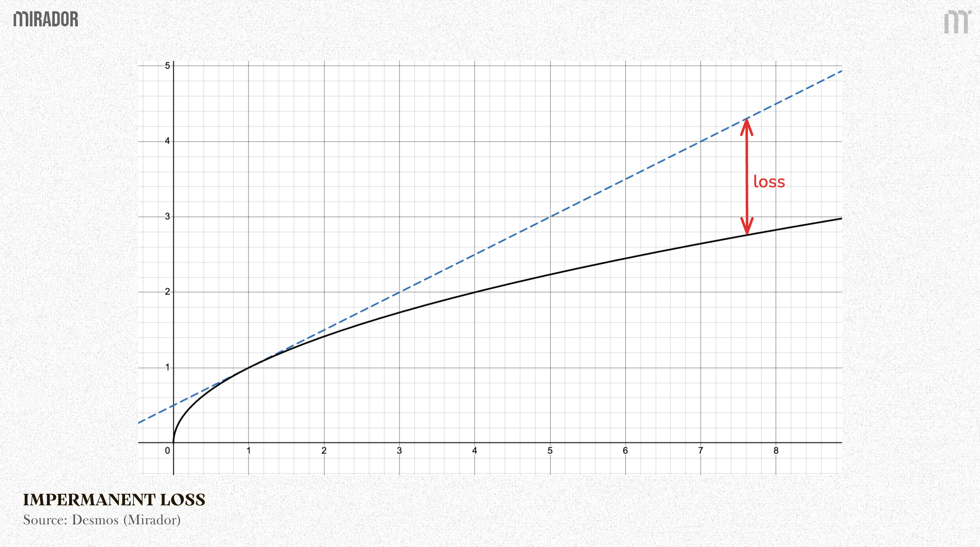
The impermanent loss stays between LP and HODL position

And converting to percentage, here’s what we got:

$IL(\%) = \frac{V_{LP} - V_{HODL}}{V_{HODL}}$

Where:

V_LP: the new value of LP position at a new token price
V_HODL: the new value of spot holding position at a new token price

But if we need to calculate the value of both HODL and LP position to work out that of IL, it would take a lot of time to reach the result. Meanwhile, the key point is that the IL only occurs when the token price changes.

So, the quickest way is to find a mathematical formula which can reflect the IL percentage through the price change only.

Let’s break them down into 2 different cases for clearer comparison.

Case 1: Simply HODL ETH and USDC in the wallet

Your wallet balance is:

x0 ETH
y0 USDC

The value of ETH balance is equal to that of USDC balance (x0*P0=y0).

And initial ETH price by USDC = P0 = y0/x0

Then, the initial total value is:

$V_0 = x_0 \cdot P_0 + y_0$

As ETH price changes (up or down), the new ETH price is P1, where:

$P_1 = k \cdot P_0$

(k = price change ratio; k≠0)

With the token balance unchanged, the new portfolio value will be:

$V_{HODL} = x_0 \cdot P_1 + y_0 = x_0 \cdot k \cdot P_0 + y_0$

$= x_0 \cdot P_0 \cdot (k + 1) \quad [1]$

Case 2: LP in a Uniswap V2 pool - 50/50 ratio with no fees (hypothetical)

Your LP balance is:

x0 ETH
y0 USDC

Initially: ETH price by USDC = P0 = y0/x0

As the pool is set with 50/50 ratio of token balance, so:

$y_0 = x_0 \cdot P_0$

The initial total LP value is:

$V_0 = x_0 \cdot P_0 + y_0 = 2x_0 \cdot P_0$

As Uniswap V2 is an invariant AMM where x*y=constant

It means:

$x \cdot y = x_0 \cdot y_0$

( x,y: new ETH & USDC balance)

And the price in the pool is always:

$\frac{y}{x} = P_1 = k \cdot P_0$

This leads to:

$y = k \cdot P_0 \cdot x \quad [2]$

Now we need to solve this to find the new token amount in the pool when ETH price changes.

First, apply [2] into the invariant:

$x \cdot (k \cdot P_0 \cdot x) = x_0 \cdot (x_0 \cdot P_0)$

$\to k \cdot x^2 = x_0^2$

$\to x = \frac{x_0}{\sqrt{k}}$

Replace this value of x into [2], we have a new function:

$y = \frac{k \cdot P_0 \cdot x_0}{\sqrt{k}} = x_0 \cdot P_0 \cdot \sqrt{k} \quad [3]$

Because the new LP value after the price changes is:

$V_{LP} = x \cdot P_1 + y$

Substitute [3] into V_LP, this leads to:

$V_{LP} = \frac{x_0}{\sqrt{k}} \cdot (k \cdot P_0) + x_0 \cdot P_0 \cdot \sqrt{k}$

$= 2x_0 \cdot P_0 \cdot \sqrt{k} \quad [4]$

As defined in the above formula:

$IL(\%) = \frac{V_{LP} - V_{HODL}}{V_{HODL}}$

Let’s replace [1] and [4] into the above IL formula:

$IL = \frac{2x_0 \cdot P_0 \cdot \sqrt{k} - x_0 \cdot P_0 \cdot (k+1)}{x_0 \cdot P_0 \cdot (k+1)}$

$= \frac{2\sqrt{k} - (k+1)}{k+1}$

Rewrite this formula, here’s the final formula:

$IL = \frac{2\sqrt{k}}{k+1} - 1$

Now, we will try using this official formula to work out the IL percentage by the price change ratio of ETH.

In the first example, we assumed the ETH to increase from $3,000 to $4,000. It means:

$k = \frac{4{,}000}{3{,}000} = \frac{4}{3} \approx 1.3333$

So:

$IL = \frac{2\sqrt{1.3333}}{1.3333 + 1} - 1 = -0.01025 \approx -1.03\%$

(exactly the same as the above result)

That’s how we check the IL via the token price change ratio without the need of working out different positions’ value. And the IL curve will look like this in a graph, as reflected by Uniswap below.

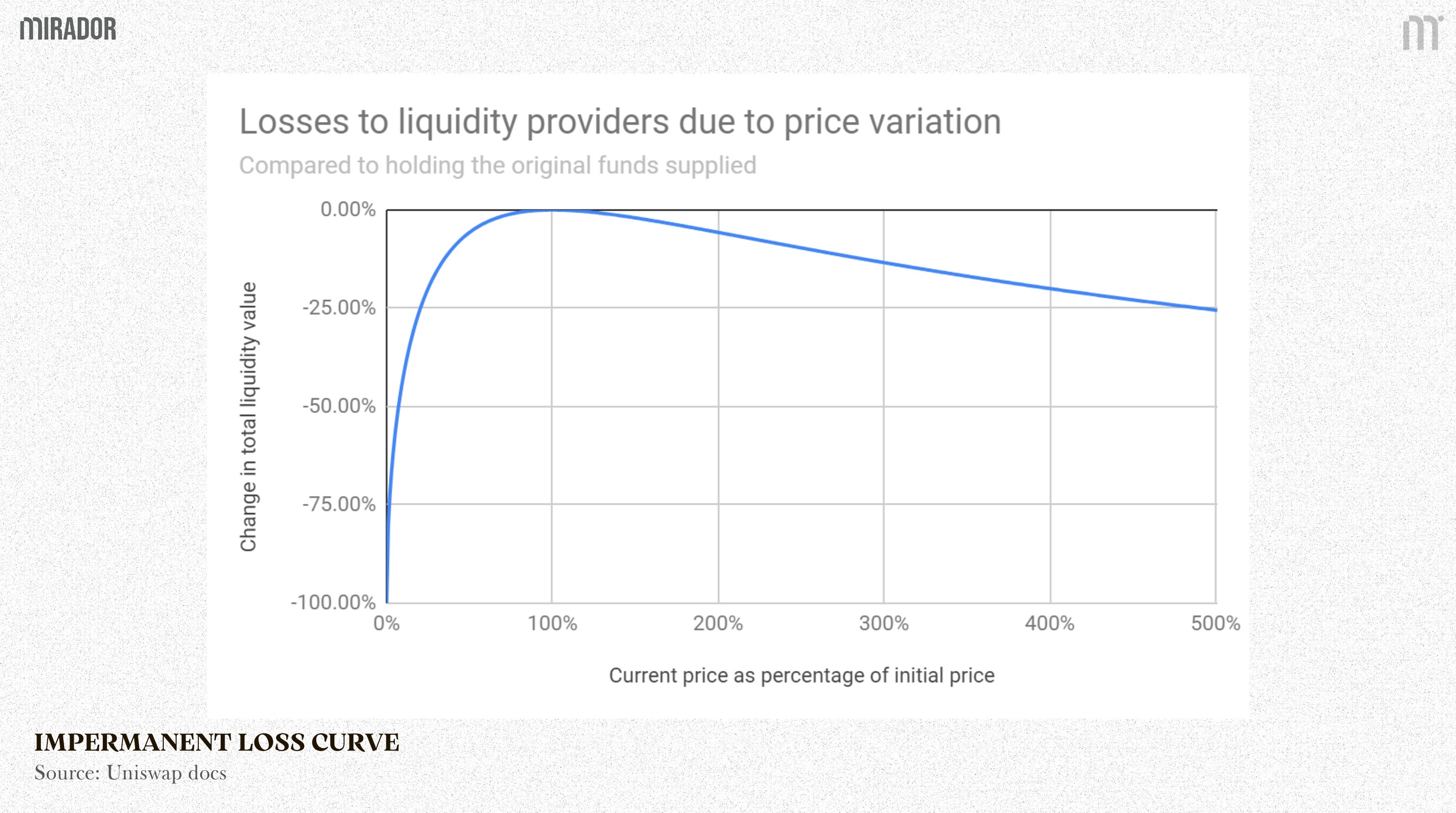
Source: Uniswap docs

Obviously, higher volatility leads to greater impermanent loss, an unavoidable cost for AMM LPs. Although it cannot be removed, it can be hedged, an approach GammaSwap enables by turning LP exposure into tradable volatility positions.

SECTION 2: THE SOLUTION - HEDGING IMPERMANENT LOSS ON GAMMASWAP

1/ What is GammaSwap?

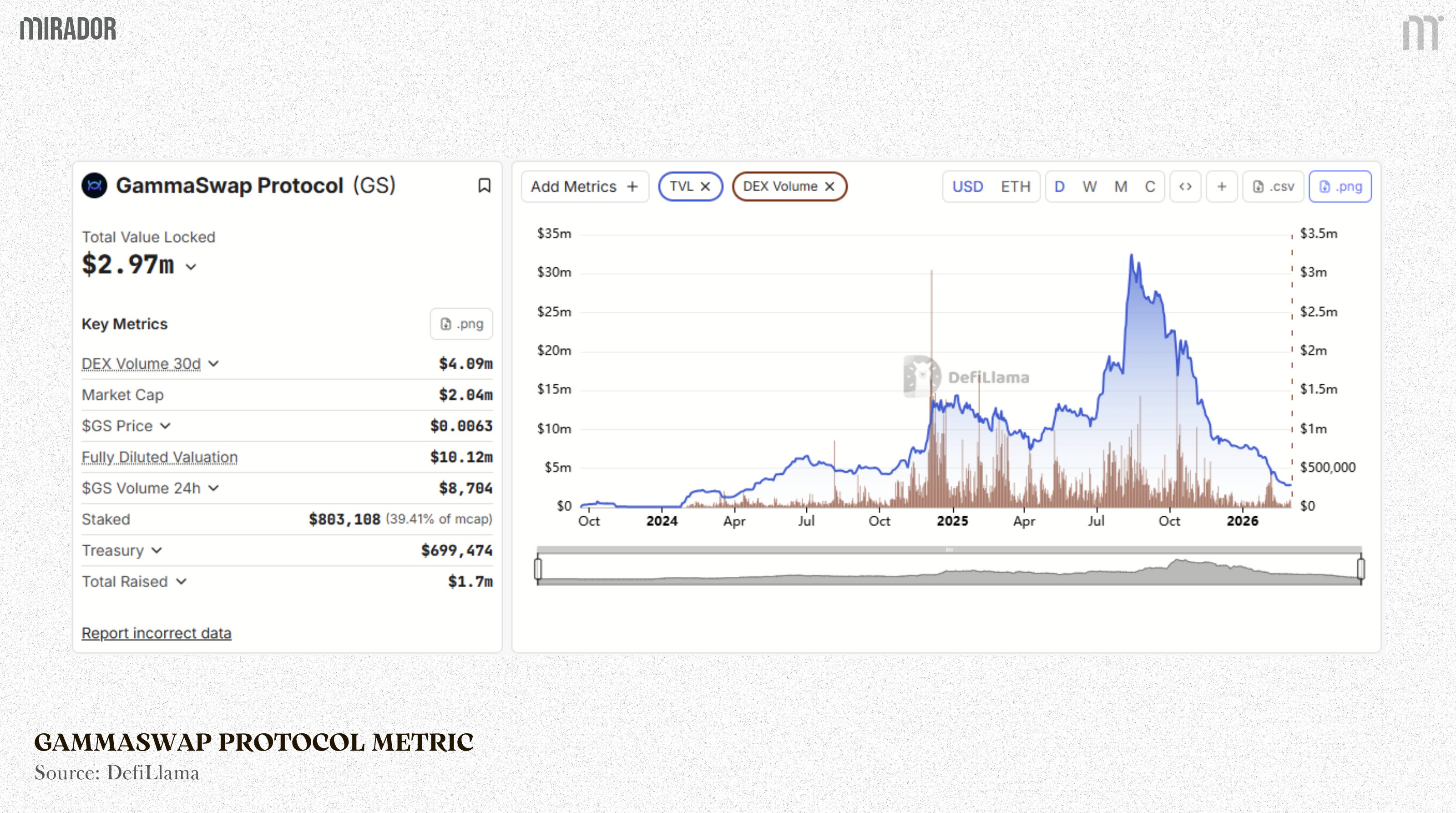
Source: DefiLlama

GammaSwap protocol is an on-chain perp options DEX launched in 2023, founded by Daniel Alcarraz, Roberto MarTinez and Devin Goodkin. In August 2025, this DEX’s total value locked (TVL) has reached its all-time high value at over $30M. Even though the TVL of GammaSwap, currently around $3M, is quite low, it doesn’t mean this protocol is a failure.

As a niche market allowing volatility trading (betting on the token price fluctuations) primarily via AMM liquidity and earning fees as an LP, in order to use GammaSwap, users need to learn about its products, especially main features on this DEX.

Simply put:

If you think the price will fluctuate significantly (up or down) → use GammaSwap to open positions by borrowing liquidity from an available AMM pool (comes with borrow rates) and earn a profit
If you think the price will be less volatile → you can act as a LP for others to “bet” on, earning swapping fees but may suffer from IL.

In terms of perp options trading, users on this DEX can trade the volatility of assets by borrowing liquidity from an AMM pool (primarily DeltaSwap - a Uniswap-like pool of GammaSwap). There are 2 main kinds of positions which traders can choose to open.

Straddle: Bet the token in the pool will be highly volatile

A straddle order on GammaSwap is a borrowed LP position where collateral is drawn at a 50:50 ratio between two tokens in the pool (the opposite of normal liquidity supply). In other words, the trader “borrows” LP tokens and exchanges them for two equal underlying assets without a need of rebalancing collateral. This position can be understood as Long Volatility position (but not the same as the directional Long below).

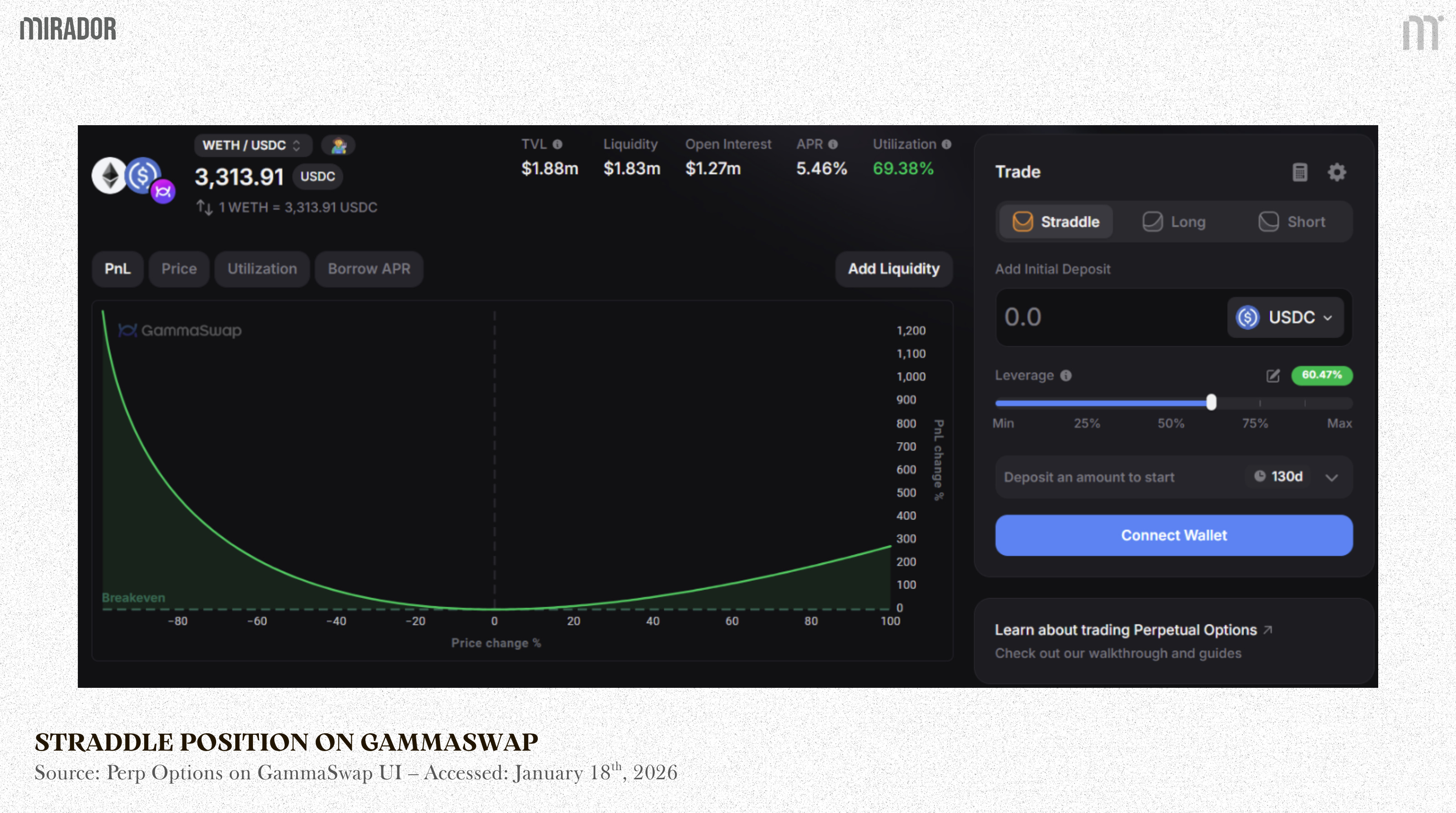
If you expect the token price to pump or dump sharply (high volatility) but you don’t know which direction (profitable either up or down), you can create a Straddle position, pay daily borrowing cost (also known as theta). If theta is lower than the price change, you earn a profit, and vice versa.

This position is suitable when the market is about to have major events (such as big news), or you want to hedge IL for your LP position because Straddle is the perfect “opposite” of LP, which can be implied as Short Volatility (but not the same as the directional Short below).

Example:

The price of ETH is currently $3000, and tomorrow, FED is going to announce future interest rates. As a trader, you believe that after or even before the news is announced, ETH will definitely fluctuate. Then, you can open a Straddle.

If the price pumps to $4000 or dumps to $2000, you make a large profit. But if it remains stable, you lose money slowly due to the borrow rate which you must pay to the LPs.

This position can be used to hedge IL in case you are an LP, too. In the next section, we will dive more into this.

B) Directional (Long/Short): Bet on the price direction, similar to Call/Put in traditional Options but different from Perp Futures

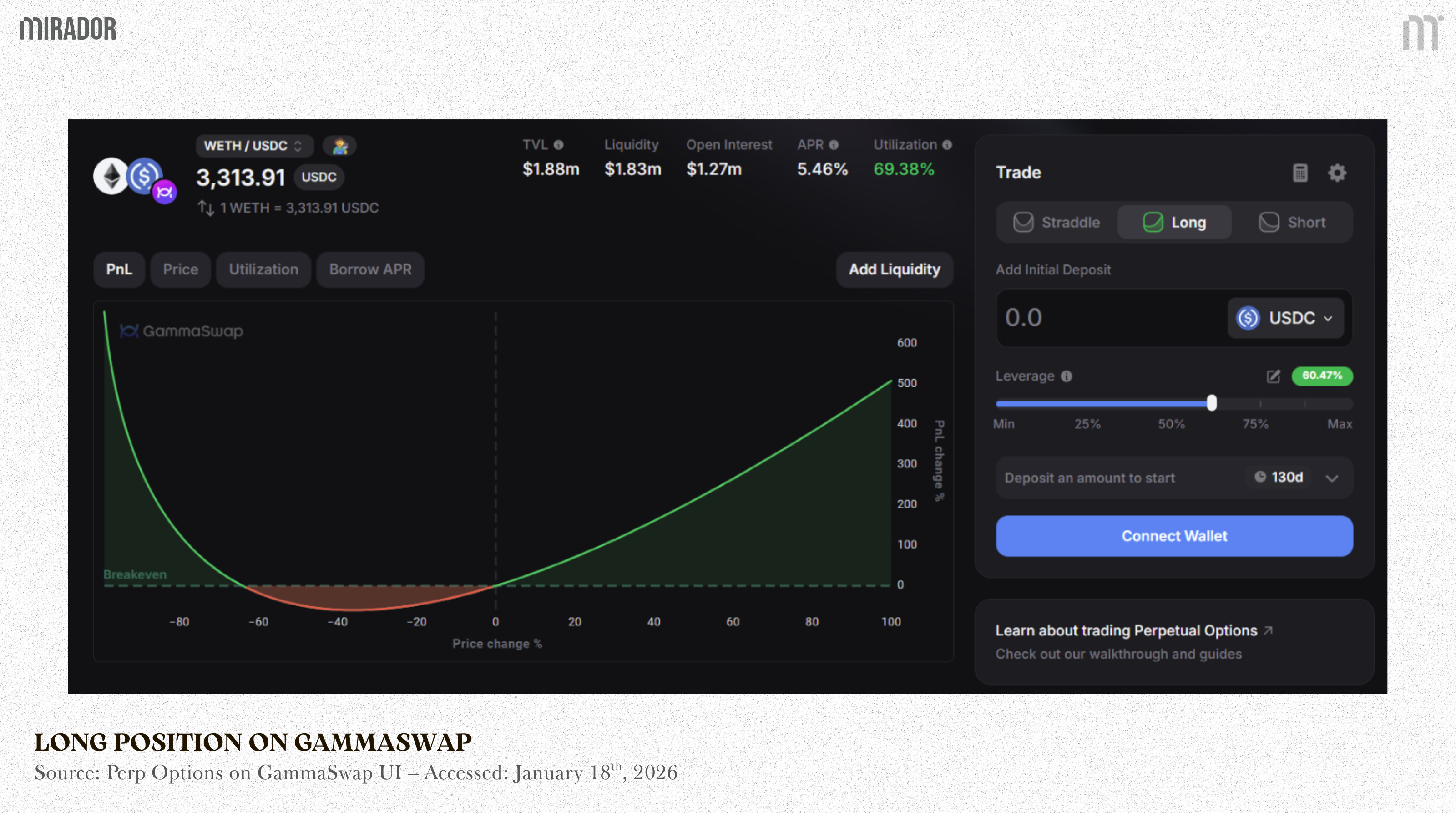
If you have a clear view on the direction of a token, you can open a Long to bet up or Short to bet down, but still benefit from volatility. This may sound like Perp Futures positions on other DEXs, but in fact, a long position on GammaSwap can still yield high profits even when the token drops sharply as reflected in the picture above. The remaining position (Short) is still similar.

Example:

You are bullish on ETH, opening a Long position at 3000. If Price goes up to 4000, you’ll get a quick profit. If it dumps to 2000, you will lose initially, but if volatility is high, GammaSwap can help reduce losses or even make a small profit.

Unlike Straddle, creating a directional position requires you to borrow liquidity and rebalance collateral to the bias ratio:

Long (Up bet): Rebalance to ~60% volatile asset (i.e, ETH) / 40% stable (i.e, USDC) → similar to Call option.
Short (Down bet): Rebalance to ~60% stable / 40% volatile → similar to Put option.

This kind of position is suitable when you are clearly bullish or bearish, but want to add leverage from volatility.

2/ How can GammaSwap solve the IL problem?

As discussed above, GammaSwap can’t completely eliminate IL but instead attempts to compensate by allowing LPs to hedge their own IL risk.

LPs can hedge IL on GammaSwap by opening a Straddle position (long gamma – volatility exposure).

In essence, traders opening a Straddle or any perp options positions on GammaSwap are borrowers, who take a liquidity loan from LPs in the AMM pool.

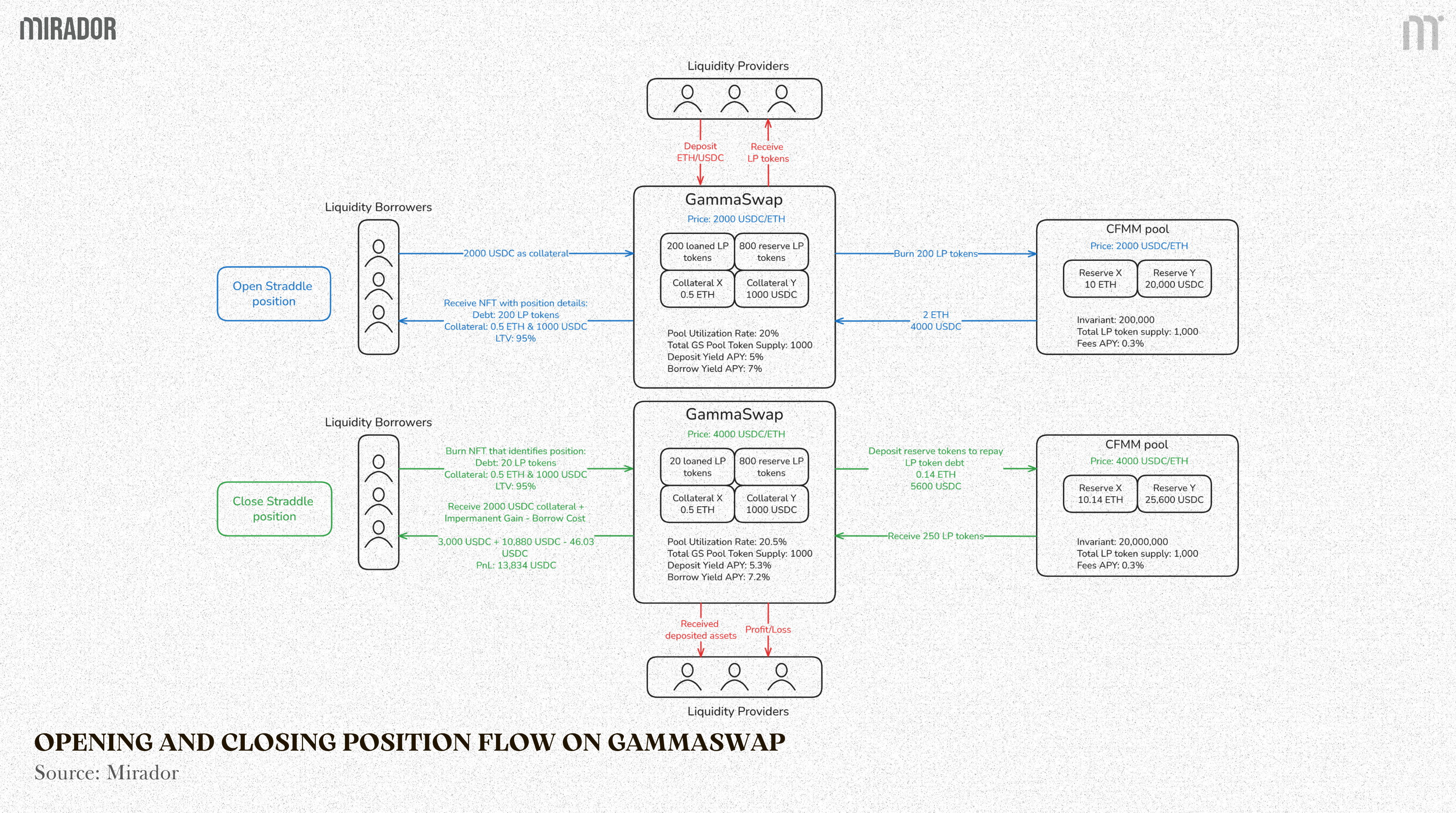
Source: GammaSwap Blog

If you want to trade the volatility (i.e. Straddle), you need to deposit your collateral (ETH + USDC) to borrow LP tokens from GammaSwap
These LP tokens will then be burnt, and you will receive reserve tokens (ETH + USDC) in the pool, which are still kept in the smart contract
Now you hold the real asset, and if the price fluctuates sharply, LP tokens will lose value due to IL but the ETH and USDC you hold in the contract are not rebalanced. Besides, you will receives an NFT (ERC-721) as a receipt for position identification in the GammaSwap smart contract
Then, when you close your position, GammaSwap will use the ETH and USDC in the contract to buy back LP tokens on AMM and your NFT will be burnt
Because LP tokens are cheaper now, you can buy more LP tokens than when you burned, and the difference value becomes your profit, or called Impermanent Gain (IG).

So the interesting point is that the more volatile the reserve tokens are, the more LP tokens can be redeemed. This is how GammaSwap turns IL into IG.

Hence, the IL is the perfect opposite of IG, or:

$IG = -IL = 1 - \frac{2\sqrt{k}}{k+1}$

(This negative calculation is like swapping LP position to HOLD position)

In our example above, we work out the result of IL as -1.03% when the ETH price pumps from $3,000 to $4,000. Applying the formula here, it means that LP will lose ~1.03% of their total token value while traders earn ~1.03% as a profit if opening a Straddle with the same position size as LP.

You can see the difference between these two parameters via the graph below, where the blue line (IG) is symmetrically opposite to the red line (IL).

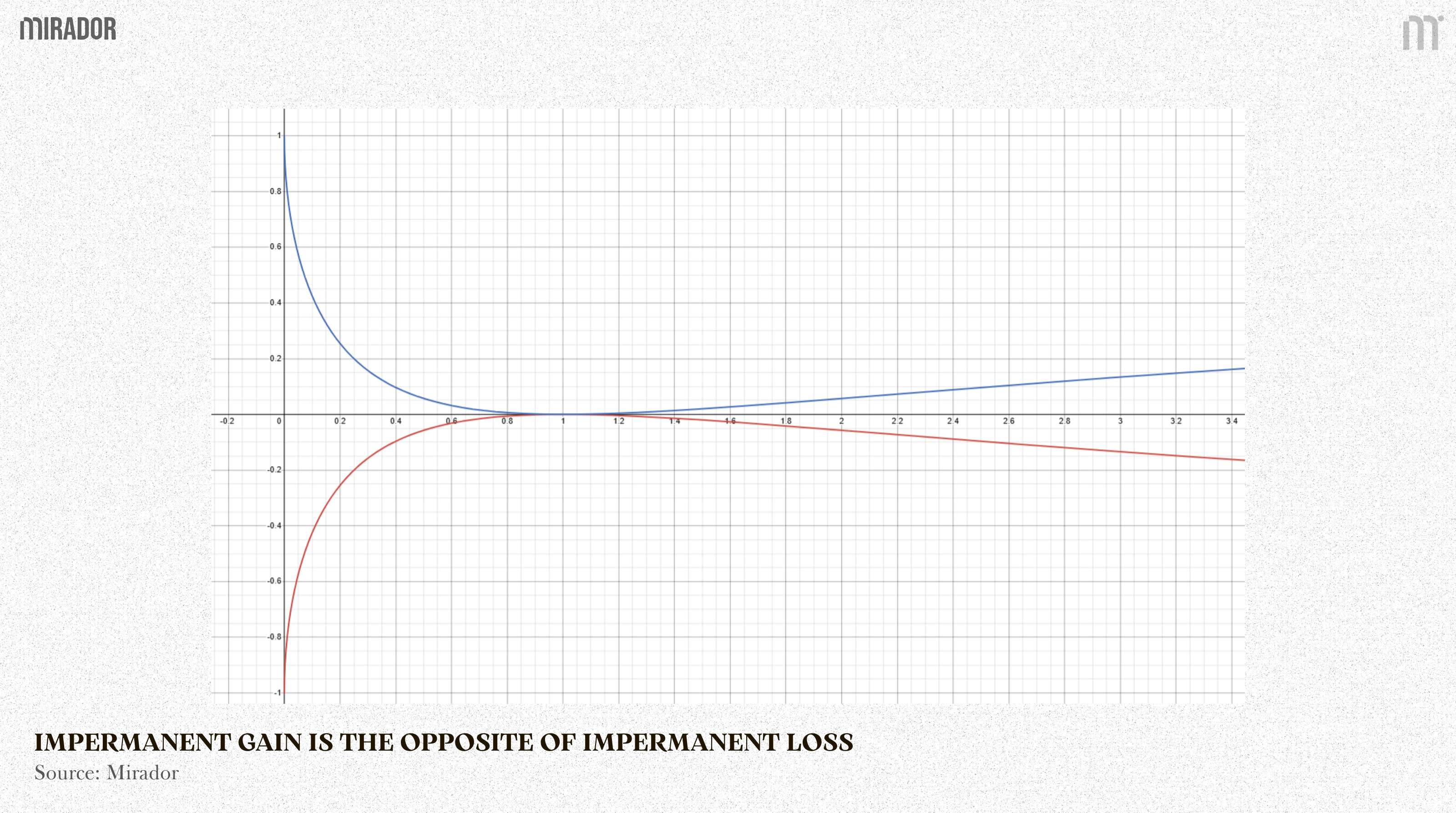
Taken together, we can see that GammaSwap is like a lending market for LP tokens, which is essentially a zero-sum game (the loss of providers is the gain of borrowers/traders).

Now, let’s examine the effectiveness of this hedging strategy via a profit simulation based on realistic figures on GammaSwap.

SECTION 3: THE SIMULATION - FEASIBILITY OF HEDGE IL STRATEGY ON GAMMASWAP

Understanding about IL, IG and how the hedging strategy works by theory is not enough but its viability must also be considered.

In this section, we will try simulating the possibility of the hedge strategy compared to LP and HODL strategy only based on realistic numbers shown on GammaSwap UI, together with the explanation behind each formula of parameters for better understanding.

On GammaSwap UI, we will try making a hedge strategy via Straddle position to work out the estimated profit with the help from GammaSwap doc.

1/ Scenarios

Let’s outline three different positions to build a profit simulation accounting model.

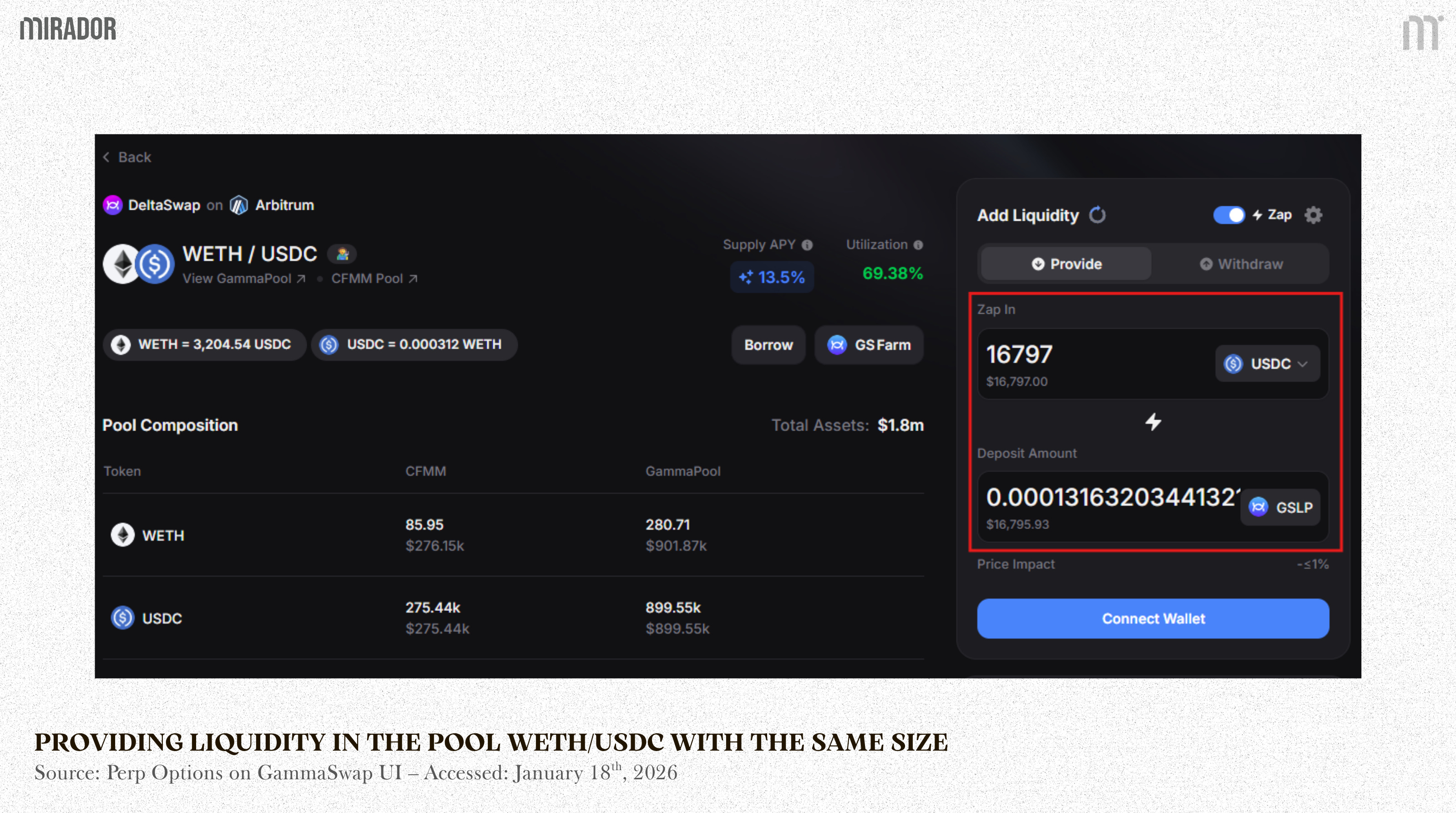
Case 1: Straddle position in the DeltaSwap pool (WETH/USDC)

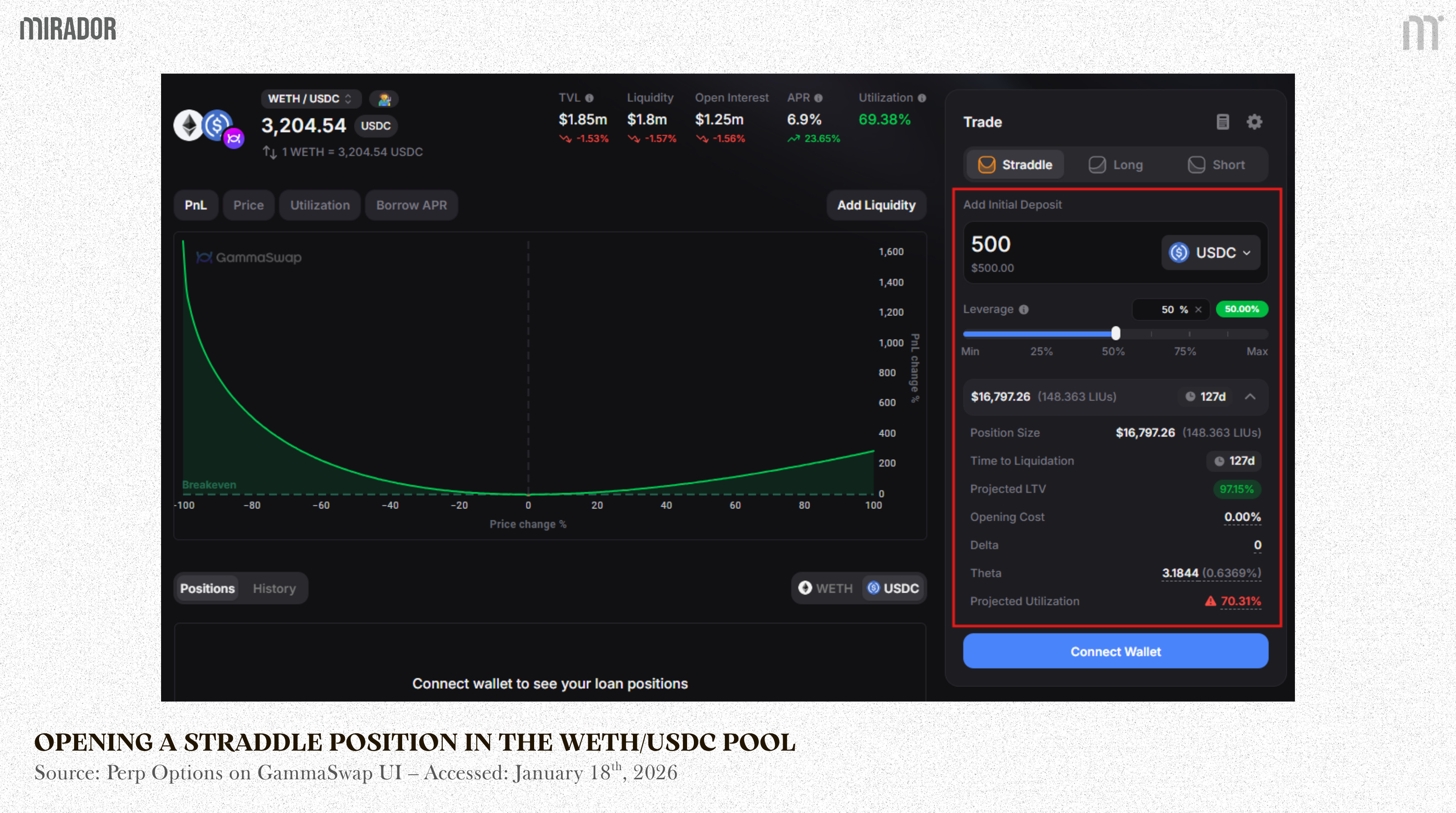
Here’s what we got from opening a Straddle position (borrowing liquidity from WETH/USDC pool) on the UI:

ETH price = $3,205
Initial deposit: $500
Leverage (Debt/collateral ratio): 50%
Position size: $16,797
LIUs (Liquidity Invariant Units): 148.363
Time to liquidation: 127 days
Projected LTV (Loan-to-Value): 97.15%
Theta (The daily cost to maintain a position): 0.6369%
Borrow rate (12h): 6.9%
LIU

For Straddle profit/loss calculation, LIU is one of the most important indicators to pay attention to since it represents the debt of the position. As traders need to borrow liquidity from the Uniswap V2-style pool with the basic invariant: x*y=k and 50:50 ratio, it means the debt value will be split equally into WETH and USDC.

Hence, here’s how we calculate the LIU:

$LIU = \sqrt{x_0 \cdot y_0} = \sqrt{x_0 \cdot x_0 \cdot P_0} = x_0 \cdot \sqrt{P_0}$

Instead of trying to find out the exact borrowed quantity of WETH and USDC, which will take a lot of time, we will just need to utilize the ETH price and position size as a quicker way.

As explained above, the new HODL position value is calculated by the following formula:

$V_1 = 2x_0 \cdot P_0 \cdot \sqrt{k} \quad [4]$

$= 2x_0 \cdot P_0 \cdot \sqrt{\frac{P_1}{P_0}}$

$= 2x_0 \cdot \sqrt{P_0} \cdot \sqrt{P_1}$

$\to V_1 = 2 \cdot LIU \cdot \sqrt{P_1} \quad [5]$

From this:

$= \frac{16{,}797}{2\sqrt{3{,}205}} \approx 148.37$

(exactly the same as LIU shown on the UI)

B) Case 2: LP in the DeltaSwap pool (WETH/USDC)

And here’s what we got when LPing into WETH/USDC pool with the same position size as Straddle:

Initial deposit: $16,797
Supply APY: 13.5%

With this initial capital and ETH price at $3,205, based on the invariant and the 50:50 ratio of the AMM pool, here’s the token balance of our portfolio:

Initial ETH: 2.62085
Initial USDC: 8,398.63

In the first case, we deposit $500 to open a Straddle position of $16,797. In this case, however, if we only provide liquidity without opening any perp options (straddle) orders on GammaSwap, our LP strategy needs to include the initial deposit which is supposed to stay in your portfolio.

In other words, LP strategy is the total equity of your portfolio in case of providing liquidity only (no hedge).

Hence:

$LP\ Strategy = LP\ Position + Initial\ Deposit$

$= \$16{,}797 + \$500 = \$17{,}297$

C) Case 3: HODL ETH and USDC spot position

In case you hold ETH and USDC spot position only, with the same token balance as follows:

Initial ETH: 2.62085
Initial USDC: 8,398.63

Your initial total portfolio value is:

$Total\ Spot\ Holdings = Initial\ Deposit + Initial\ HODL\ position\ value$

$= \$500 + 2.62085 \cdot 3{,}205 + 8{,}398.63$

$= \$500 + \$16{,}797 = \$17{,}297$

2/ How to calculate Straddle PnL?

The success of hedging IL strategy depends on the profitability of Straddle position. If the IL of a LP is $5, in order to compensate this loss, a straddle position should make an IG of $5, too.

To calculate the profit/loss (PnL) as well as IG, we compare the current portfolio value with the portfolio value at the time the position was opened. In other words, the current PnL of the position will be the difference between the current and initial portfolio values.

$PnL = V - V_0$

Where:

V: The portfolio value at the current time
V0: The portfolio value at the initial time

A Straddle position on GammaSwap is essentially a portfolio consisting of short LP tokens and buying the underlying tokens that the LP token represents (i.e. WETH & USDC).

Therefore, the position value at the current time is the difference between the token value you are currently holding and LP token value you are borrowing.

$V = V_{HODL} - V_{LP}$

Replace [5] into V:

$\to V = x \cdot P + y - 2 \cdot LIU \cdot e^{rt} \cdot \sqrt{P}$

Where:

x: the quantity of the first underlying token (i.e. WETH)
y: the quantity of the second base token (i.e. USDC)
P: the current price of the first token relative to the second token (e.g., the price of WETH in USDC)
LIU: the liquidity invariant of the amount of LP tokens borrowed at the time of opening the position
t: the time (year) elapsed since the borrowing
r: annual borrow rate of LP pool
e^rt: represents the debt growth due to compounded interest

And this is the position value at the initial time (t=0):

$V_0 = x \cdot P_0 + y - 2 \cdot LIU \cdot \sqrt{P_0}$

Replace the V and V0 formula into the PnL’s above. Here’s the final result:

$PnL = x \cdot (P - P_0) - 2 \cdot LIU \cdot \left(e^{rt}\sqrt{P} - \sqrt{P_0}\right)$

NOTE:

In this simulation model, we assume t=0 in order to isolate price-driven effects and evaluate the effectiveness of IL hedging. Time-dependent factors such as borrow rates (r) and time to liquidation (t) are therefore excluded from the model.

So, in this case:

$Straddle\ PnL\ (\$) = x \cdot (P - P_0) - 2 \cdot LIU \cdot \left(\sqrt{P} - \sqrt{P_0}\right) = IG$

Now, we shall apply this formula for hedge strategy simulation below.

3/ Hedging IL Strategy - Simulation Results

A successful hedge strategy is one where its return equals that of spot holdings and the IL of LPs can become the IG of traders (or the LP themselves if they open a trade). So, our goal is to make:

$HEDGE = LP + Straddle \approx HODL$

$And:\ IG = -IL$

no matter how ETH fluctuates.

Now, it’s time to dive in the accounting model. Below is our result of the hedge strategy’s returns compared to LP and HODL only.

Where:

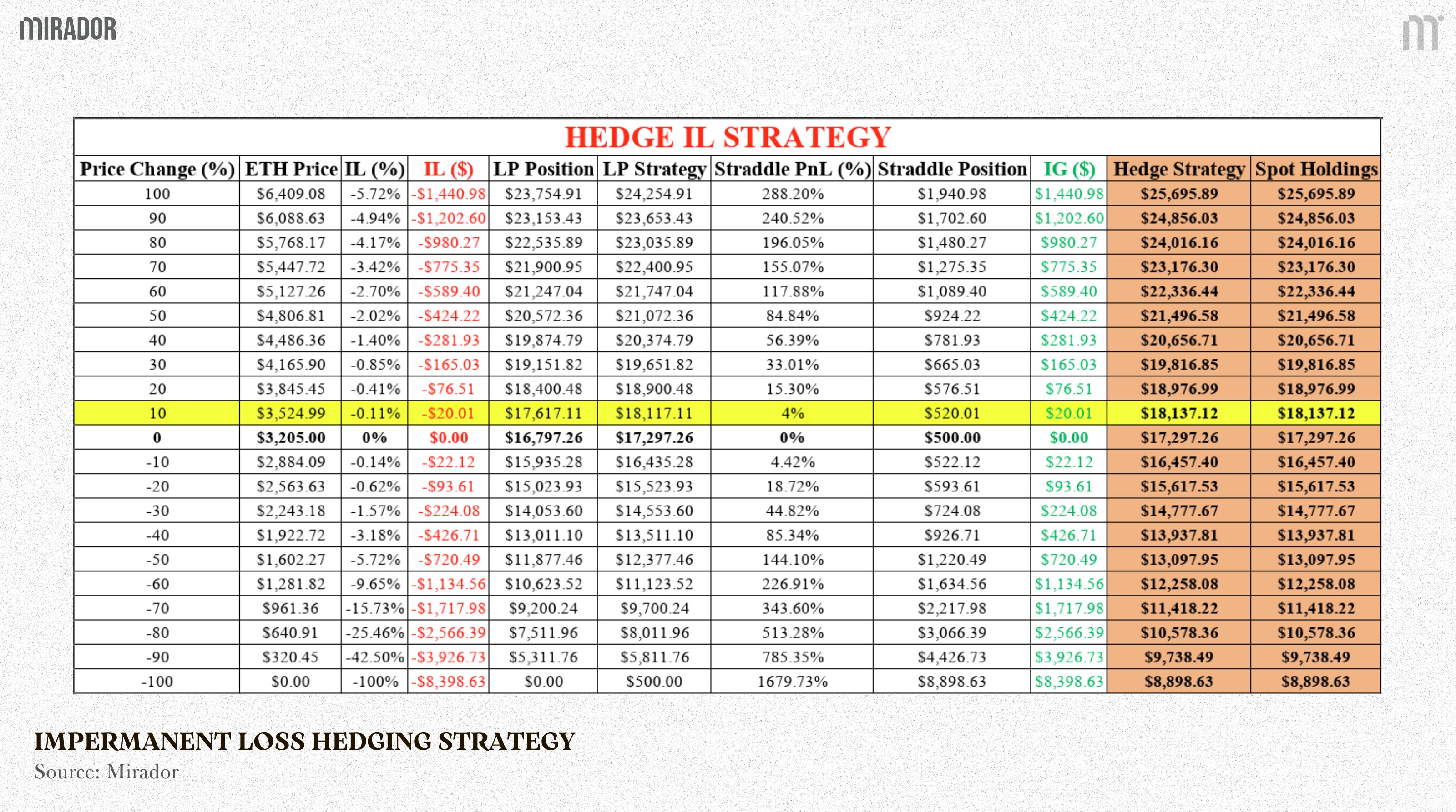
$IL(\%) = \frac{2\sqrt{k}}{k+1} - 1 \qquad \{k = \frac{\text{new ETH price}}{\text{initial ETH price}}\}$

$IL(\$) = LP\ Strategy - Spot\ Holdings$

$LP\ position = (Initial\ ETH\ balance \cdot ETH\ price + Initial\ USDC\ balance)\cdot(1+IL)$

$LP\ Strategy = LP\ Position + Initial\ Deposit$

$Spot\ Holdings = Initial\ deposit + Initial\ ETH\ balance \cdot ETH\ price + Initial\ USDC\ balance$
$Straddle\ PnL\ (\$) = Initial\ WETH\ balance \cdot (New\ ETH\ price - Initial\ ETH\ price) - 2 \cdot LIU \cdot \left(\sqrt{New\ ETH\ price} - \sqrt{Initial\ ETH\ price}\right) = IG(\$)$

$Straddle\ PnL\ (\%) = \frac{Initial\ WETH\ balance \cdot (New\ ETH\ price - Initial\ ETH\ price) - 2 \cdot LIU \cdot \left(\sqrt{New\ ETH\ price} - \sqrt{Initial\ ETH\ price}\right)}{Initial\ Deposit}$
$Straddle\ position = Initial\ deposit + Straddle\ PnL\ (\$)$
$Hedge\ Strategy = LP\ position + Straddle\ position$

Example:

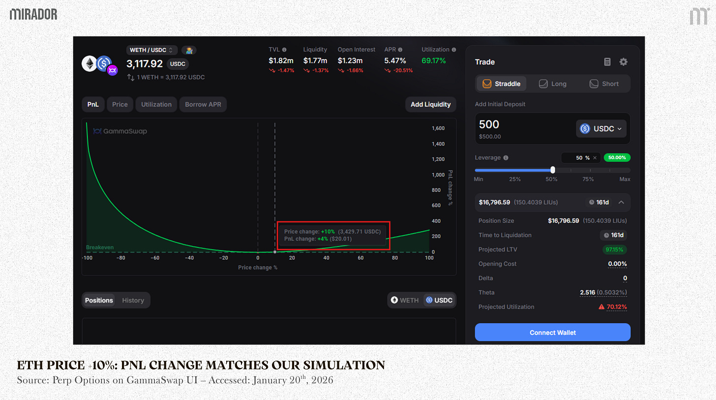
At a price increase of 10% for ETH ($3,524) (yellow-highlighted row), here’s the result of these parameters:

$IL = \frac{2\sqrt{1.1}}{1.1+1} - 1 = -0.11\% \qquad \left\{k = \frac{\text{new ETH price}}{\text{initial ETH price}} = \frac{3{,}525}{3{,}205} = 1.1\right\}$
$LP\ position = (Initial\ ETH\ balance \cdot ETH\ price + Initial\ USDC\ balance)\cdot(1+IL) = (2.62085 \cdot 3{,}525 + 8398.63)\cdot(1-0.11\%) = \$17{,}617$
$LP\ Strategy = LP\ Position + Initial\ Deposit = \$18{,}117$

$Spot\ Holdings = Initial\ deposit + Initial\ ETH\ balance \cdot ETH\ price + Initial\ USDC\ balance = \$500 + 2.62085 \cdot 3{,}525 + 8398.63 = \$18{,}137$
$IL(\$) = LP\ strategy - Spot\ holdings = \$18{,}117 - \$18{,}137 = -\$20$
$Straddle\ PnL\ (\$) = 2.62085 \cdot (3{,}525 - 3{,}205) - 2 \cdot 148.363 \cdot \left(\sqrt{3{,}205} - \sqrt{3{,}205}\right) = \$20 = IG = -IL$

$Straddle\ PnL\ (\%) = \frac{\$20}{\$500} = 4\% \qquad \text{(aligned with the PnL change shown on the UI in the picture below)}$
$Straddle\ position = Initial\ deposit + Straddle\ PnL\ (\$) = \$500 + \$20 = \$520$
$Hedge\ Strategy = LP\ position + Straddle\ position = \$17{,}617 + \$520 = \$18{,}137 = Spot\ Holdings$

Applying the same formulas to other ETH price cases, it’s obvious to see that the more ETH price fluctuates, straddle position always earn higher profit than LP and HODL.

Specifically, looking at the IL, IG and two orange-highlighted columns, we can clearly see that the IL of LP has become the IG of straddle traders, making the hedge strategy equal to HODL strategy.

Or, it also means that the loss that LPs suffer from LP strategy can be compensated by opening a Straddle position with the same size to hedge and make it their profit gain. Adding it all up, LPs will suffer from no loss (IG + IL = 0) and then, their realized profit depends on their swapping fees.

So, from the above mathematical results, we can draw out a line graph to compare as below.

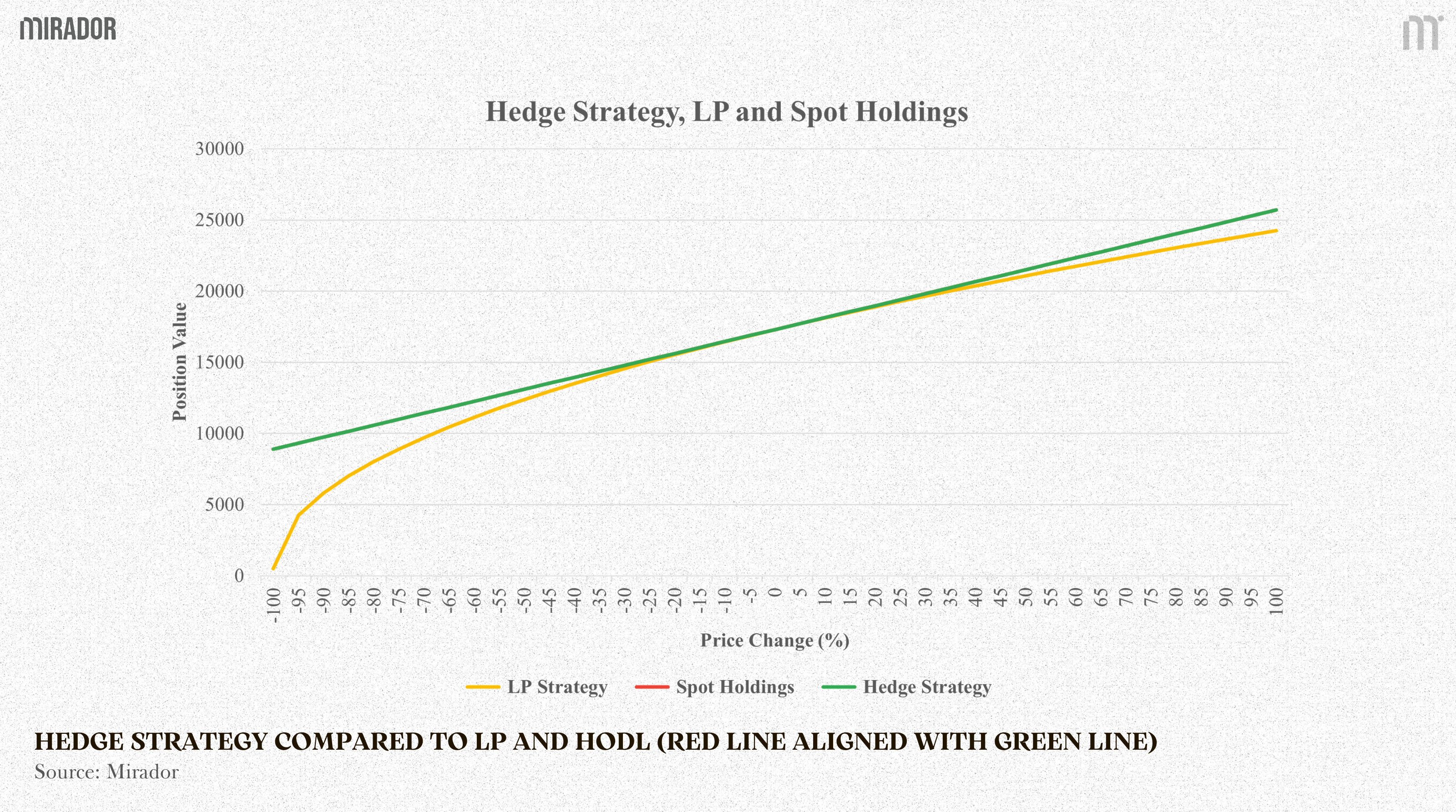
In this graph, you can’t see any particular lines for spot holdings because the return of hedge strategy (green line) is completely aligned with that of spot holdings (red line), whereas LP strategy is a downward curve (yellow curve) due to the impact of IL.

From the detailed simulation of the accounting model as explained above, together with all these assumptions based on realistic numbers on GammaSwap UI, the hedge strategy can be made successful to turn the impermanent loss of LP into the impermanent gain of traders. In simple terms, LPs can use this strategy to hedge their unavoidable IL and earn a positive profit from their borrow fees.

Yet, please note that actual results on GammaSwap may vary due to market conditions, funding dynamics, liquidity, and protocol-specific risk parameters. The above is our simulation based on real-world parameters, and it could become a reality if the price of ETH fluctuates significantly, as in the scenarios where these assumptions change.

CONCLUSION

While real-world outcomes may vary depending on market conditions and execution, the analysis and simulations above suggest that GammaSwap offers a compelling approach to managing impermanent loss. Impermanent loss is an inevitable event that every liquidity provider has experienced. Although it’s impossible to completely eliminate this loss, through GammaSwap, this exposure can be actively hedged, and under favorable market conditions, even transformed into a source of profit.

Disclaimer

This article focuses on explaining the mathematical design and core mechanics behind GammaSwap, particularly how impermanent loss can be hedged and transformed into impermanent gain through LP-based volatility positions. The analysis is intended to clarify the underlying logic of the protocol rather than to evaluate performance, compare protocols, or recommend specific trading strategies.

All models, formulas, and simulations presented are simplified in order to illustrate key concepts under idealized assumptions. Actual results on GammaSwap may vary due to market conditions, funding dynamics, liquidity, and protocol-specific risk parameters. This article is for educational purposes only and should not be considered financial or investment advice.

Ahead of the GammaSwap V2 launch, we will return with further deep-diving articles exploring other key components of the new architecture.

Discussion about this post

Ready for more?