

GAMMASWAP: THE BASIS OF “GAMMA SWAPPING” THROUGH PERPETUAL OPTIONS
A structural introduction to gamma exposure, impermanent loss, and how GammaSwap’s perpetual options enable gamma hedging

INTRODUCTION
GammaSwap is an on-chain perpetual options protocol launched in 2023 with a clear promise: to hedge impermanent loss.
But its concept also left new users confused: “What is gamma?”, “What does “Gamma Swap” mean?”, “Why does swapping gamma help reduce impermanent loss?” and “How does this work through perpetual options?”.
In this article, we focus on answering these questions in the simplest and most fundamental way, explaining the core ideas behind gamma, impermanent loss, and how GammaSwap connects them.
KEY TAKEAWAYS
Section 1: Gamma explains why exposure changes with price, and why swapping gamma means trading volatility instead of direction.
Section 2: Impermanent loss is simply negative gamma embedded in AMM liquidity provision.
Section 3: GammaSwap turns this gamma exposure into perpetual options for hedging and volatility trading.
Writer’s note:
This article connects option models in both DeFi and traditional finance, and includes some mathematical ideas (fully simplified). We recommend reading it patiently, step by step, starting from the fundamentals. Each section builds on the previous one, and the full picture only becomes clear when the pieces are put together.
***
“Gamma” is not specific to GammaSwap, it comes from a broader framework used to describe risks of a financial position.
Gamma is part of the most the most powerful analytical tools - the Option Greeks. They are a set of financial measures, designed to quantify risk and show how an option’s price responds to changes in market conditions, where delta and gamma describe how an option’s price responds to price movements in the underlying asset.
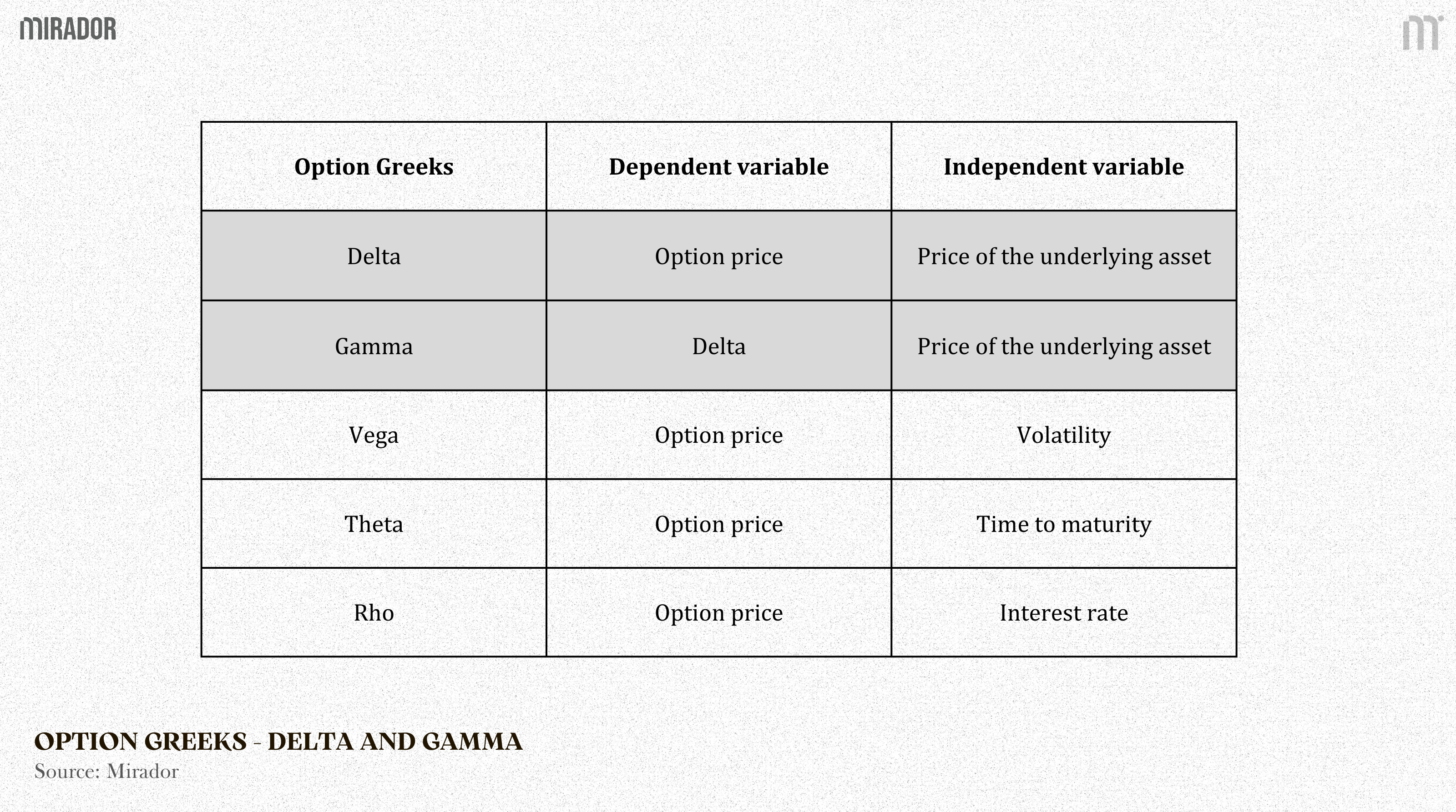
In practice, Greeks measures are most commonly used in options trading (Option Greeks).
An option is a contract that gives you the right to buy or sell an asset at a predetermined price.
The cost of buying an option (option premium) represents the market’s expectation of how much the underlying asset will move. You make a profit if the asset moves more than what is priced in, and you lose money if the asset does not move, or moves too little to justify that cost.
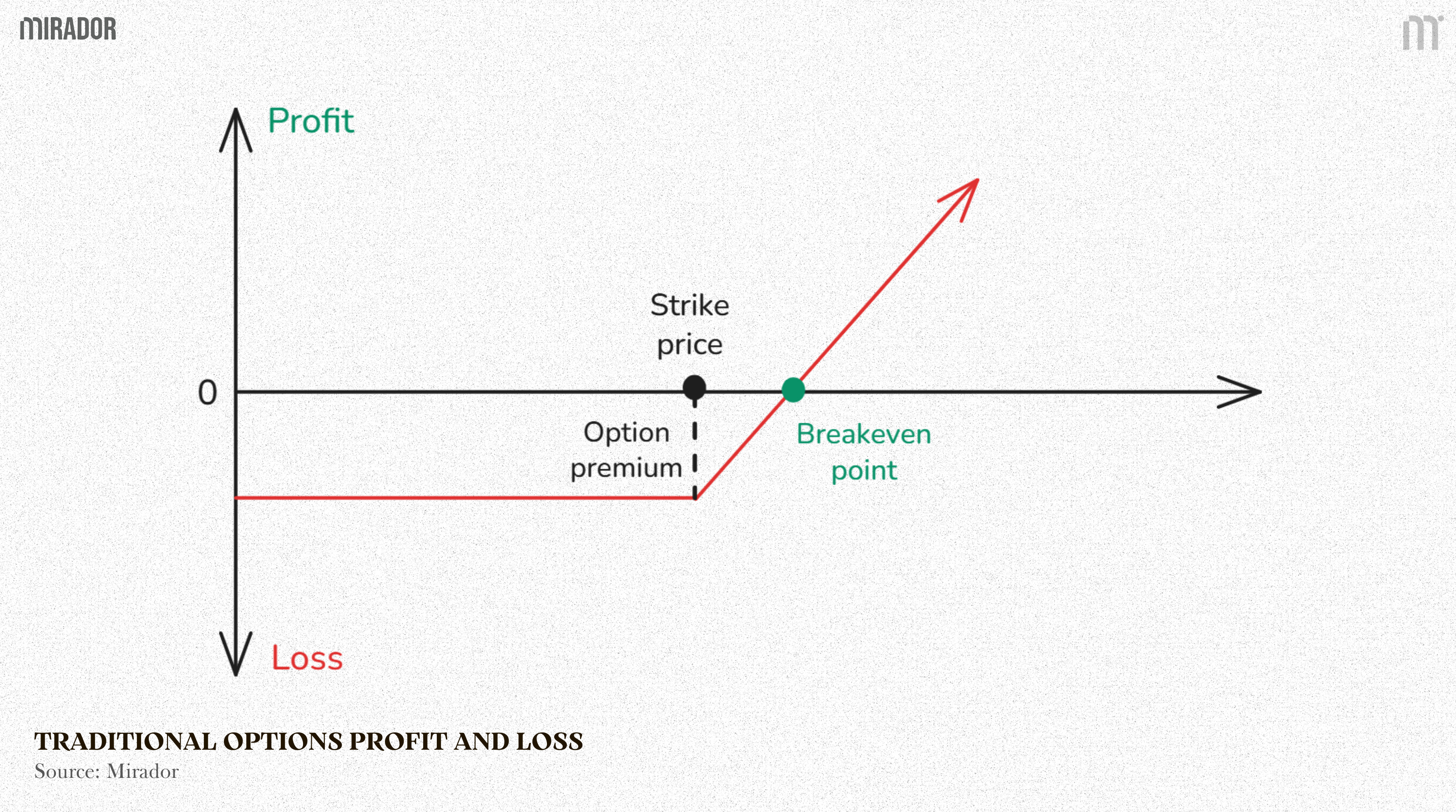
Suppose you buy a call option with a strike price of $34,000 (the right to buy asset at price of $34,000 on expiration day), and you pay an option premium of $200.
This $200 is the maximum loss you can incur. If the price stays below the strike, the option expires worthless and you lose the premium.
The breakeven price is the strike plus the premium. In this case, breakeven is $34,200.
Here is how profit and loss work:
If the asset price is below $34,000, you do not exercise the option. Your PnL stays at –$200.
If the price moves above $34,200, you start making money.
Traditional options have an expiration date, which means your opportunity to profit is limited to that timeframe.
A perpetual option removes this time limit, it gives the holder the right to exercise at any moment, without an expiration date. This is the concept used in GammaSwap, offering full flexibility to buy or sell the underlying asset whenever it becomes strategically favorable.
In the first two section, we use delta and gamma as general tools for measuring risk across different financial positions (not only option). By doing so, we can better understand their underlying meaning, and ultimately see what “gamma swap” through “perpetual option” really refers to.
SECTION 1: GAMMA AND “GAMMA SWAP”
Gamma is often mentioned as if it stand alone, but in reality, gamma cannot be understood without first understanding delta.
Among these Greeks, one describe what your exposure is, while the other describe how that exposure changes.
1/ Delta - the root of Gamma
Fixed delta (future contract)
Delta measures how sensitive an option’s value is to price changes in the underlying. In simple terms, it tells you how much the option’s price is expected to move when the underlying price moves by $1.
This sensitivity represents your price exposure - how strongly your position reacts to market movements.
In a futures position, your exposure does not change as the price moves, every $1 movement in the underlying always results in the same $1 gain or loss. In other words, delta stays constant across all price levels (fixed delta).
Suppose you go long 1 BTC perpetual futures at a price of $50,000.
If the price rises to $55,000, you make $5,000.
If the price falls to $45,000, you lose $5,000.
For every $1 move in price, your profit or loss changes by exactly $1. This one-to-one relationship is what defines a linear payoff.
In this case, we have fixed delta is 1.
Put on a chart, the futures value is just a straight line.
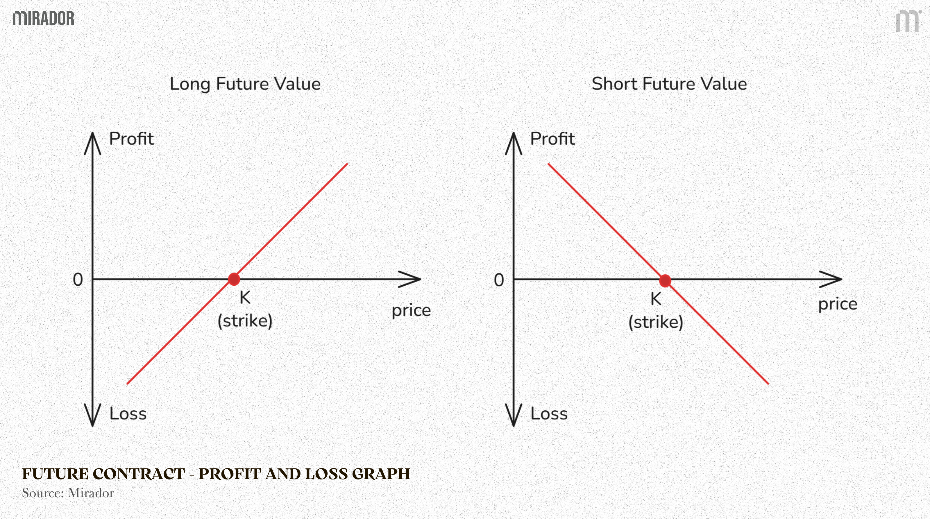
With K is strike price of a future contract
A long futures position has a straight-line PnL: you gain as the price rises above K and lose as it falls below K.
A short futures position is the exact opposite: your PnL decreases linearly as the price moves above K and increases as it moves below K.
This linear relationship remains exactly the same even when leverage is added.
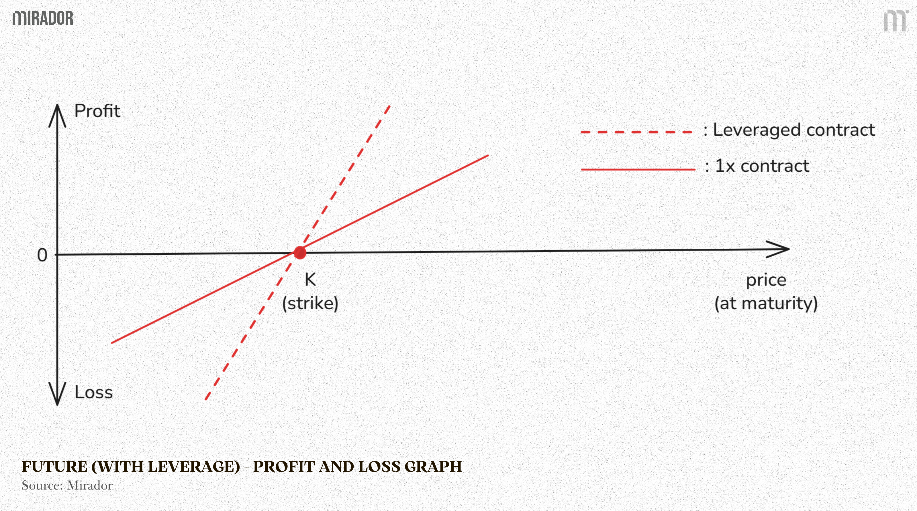
For example, if the price moves by +1%, your PnL also moves by +1% (or −1% if you’re short).
That corresponds to a delta of +1 (or −1 if the position is short).
With 5× leverage, the PnL simply scales to +5% or −5%, but the line is still perfectly straight, nothing about the shape changes.
This means the position’s delta is +5 (or −5 if short), but it is still fixed.
In conclusion, fixed delta means that the value of a contract always changes at a constant rate relative to the price of the underlying asset.
Non-fixed delta, therefore, simply means that this relationship is not constant: the sensitivity itself changes as price moves.
Non-fixed delta (option contracts) and the root of gamma
Option contract and volatility trading
The most representative example of non-fixed delta is the option contract, a product that is best understood as a trade on volatility rather than on price direction.
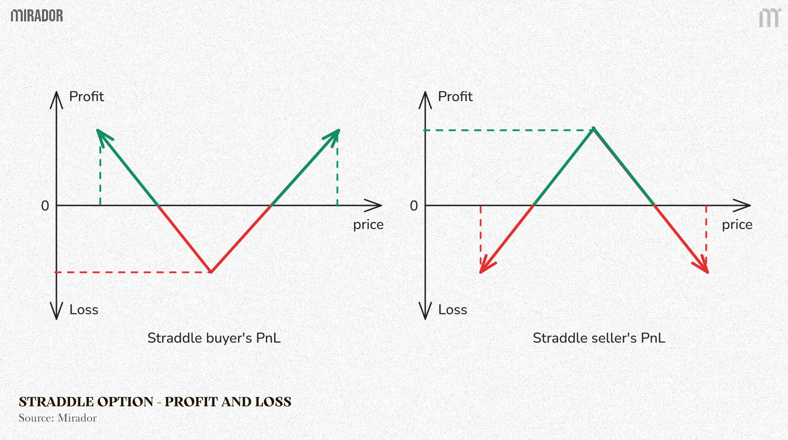
The idea of trading volatility becomes clear only when we look at option structures such as a straddle, where directional exposure is neutralized and the payoff is driven primarily by price movement itself.
But if we only consider the payoff of an option at expiration, things like delta and gamma are not really meaningful.
The diagrams below show the payoff of basic option (call/put) positions at expiration, which is still linear from breakeven price (breakeven price is strike price plus premium):
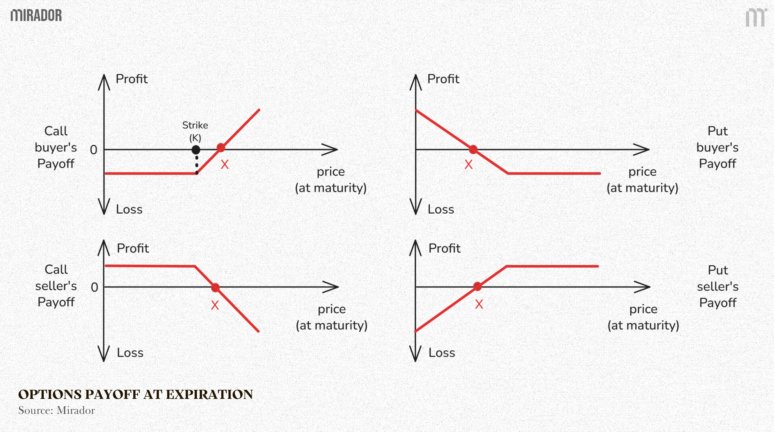
For a long call, the payoff is zero when the price stays below the strike price (explained below). Once the price moves above the strike, the payoff increases linearly as the price rises.
For a long put, the payoff increases linearly as the price falls below the strike price, and becomes zero once the price moves above it.
The short positions are simply the opposite.
However, these payoff diagrams only describe options at expiration.
In reality, what makes options interesting is that their value changes continuously before expiration. At any moment, an option’s price reflects the market’s expectation of how likely it is that the payoff will end up above zero.
Because of that expectation, with options, delta is not fixed. It changes depending on where the underlying price is relative to the strike, whether the option is out of the money (OTM), at the money (ATM), or in the money (ITM).
Out of the money (OTM): The option has no intrinsic value. A call option is OTM when the price is below the strike, and a put option is OTM when the price is above the strike. In this region, delta is close to zero because price moves have little impact on the option’s value.
At the money (ATM): The price is close to the strike. Small price changes significantly affect the probability of the option finishing in the money, so delta changes rapidly. This is where gamma is highest.
In the money (ITM): The option already has intrinsic value. A call option is ITM when the price is above the strike, and a put option is ITM when the price is below the strike. Here, delta moves closer to one (or −1 for puts), and the option starts to behave more like the underlying asset.
As the underlying price moves, that probability changes, and so does the option’s value.
This is where we should mention “non-fixed delta”.
Non-fixed delta in option
For example, suppose there is a call option with a strike price of $300.
(The strike price is the predetermined price at which holder of an option has right to buy (call option) or sell (put option) the underlying asset at expiration)
Strike price is also the reference price that determines whether the option is OTM, ATM, or ITM.
The chart below shows how the delta of this call option changes as the price of the underlying asset moves relative to the strike price.
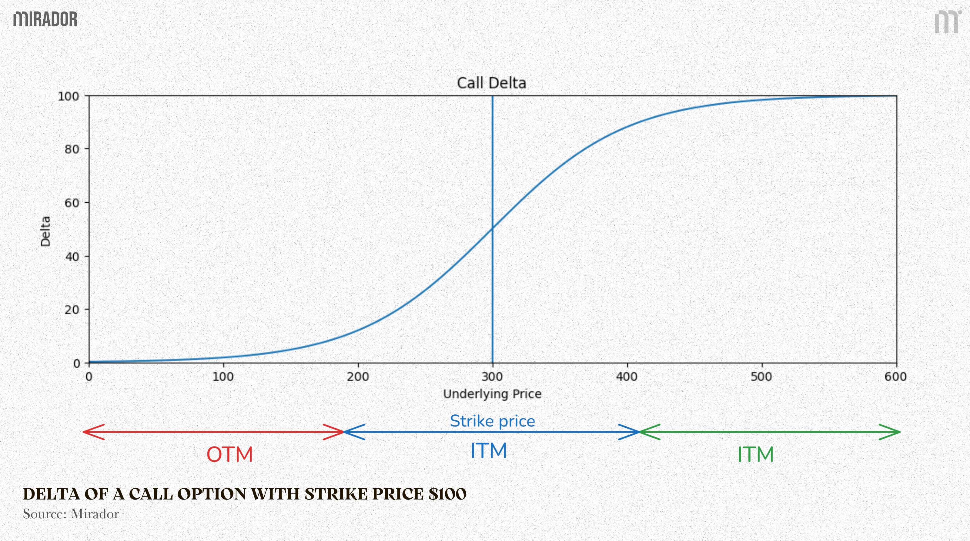
This chart shows how the delta of a call option changes as the underlying price moves.
When the price is far below the strike ($300), delta is close to 0. For example, If delta is around 0.0, this means if the underlying price increases by $1, the option price only increases by about $0.05.
As the price approaches the strike, delta increases rapidly. For example: delta may rise to 0.50. Now a $1 move in the underlying leads to roughly a $0.50 move in the option price.
Once the option is deep ITM, delta flattens out and moves close to 1.00. For example: delta can reach 0.95 or higher. At this point, a $1 move in the underlying results in almost a $1 change in the option price, making the option behave very much like the underlying asset itself.
Explanation:
When the price is far below the strike, delta is close to zero because the option has little chance of finishing in the money. As the price approaches the strike, small price moves have a much bigger impact on that probability, so delta increases rapidly.
Once the option is deep in the money, the outcome becomes more certain. The option is very likely to finish in the money, so further price moves change that probability only slightly, and delta flattens out near one.
And this is the key to identifying convexity.
What makes this behavior possible is gamma.
And now, what is “Gamma”?
Gamma measures how quickly delta itself changes as the underlying price moves.
Put another way, gamma (Γ) is the first derivative of delta (Δ) with respect to the underlying asset price (P).
With a linear payoff (fixed delta) like futures.
When the underlying price P increases by 1 unit, the position value always increases by a constant amount. As a result, delta is constant.
Since delta is a constant, its derivative with respect to price is zero => Gamma = 0
For example: If you hold a futures contract, for every P rise in price, your PnL increases by a fixed amount. Delta is always 1. The rate of change of 1 is gamma, and it’s 0.
With a non-linear payoff (non-fixed delta) like options
As the underlying price P changes, the option’s sensitivity to price (delta) also changes.
Delta is a function of price, so its derivative with respect to price is not zero => Gamma ≠ 0
For example: With a Call Option, as the price S rises, the option becomes more likely to finish “in-the-money”, causing delta to increase from 0.50 to 0.60. This rate of change is the gamma.
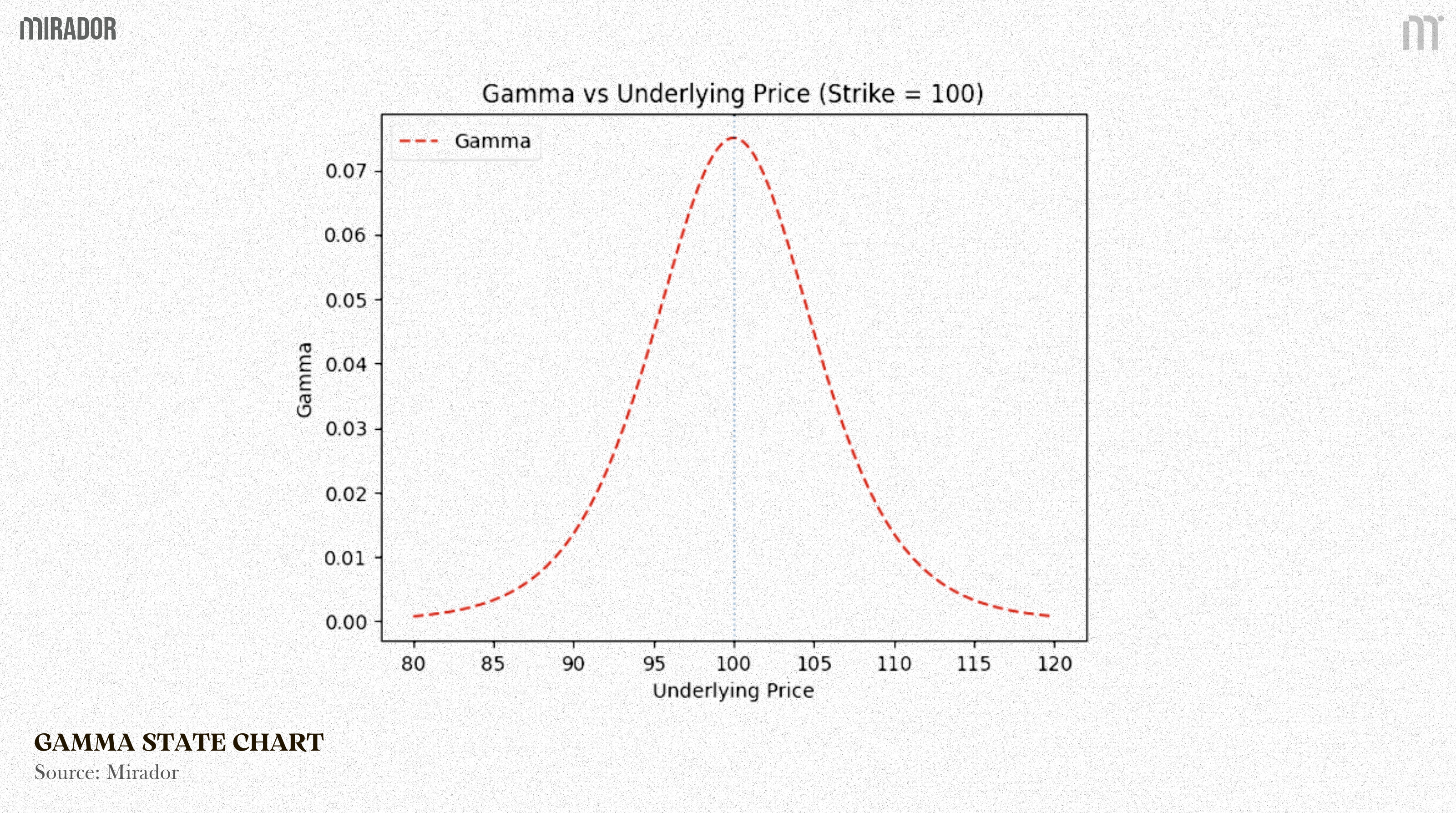
To understand the way Gamma measures how fast delta changes as the underlying price moves, let’s make a simple example:
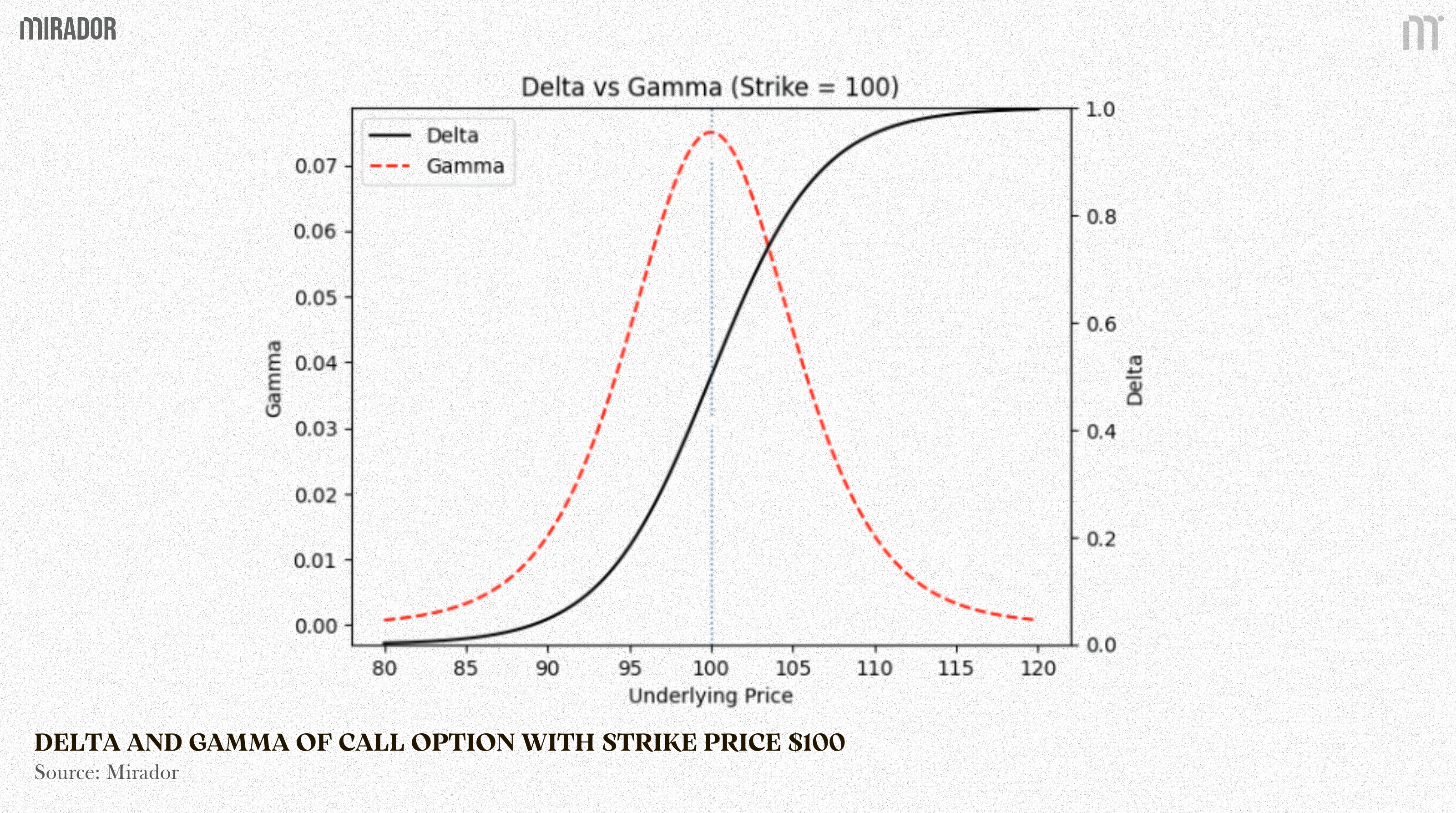
When the option is far out of the money, delta is close to zero and barely changes. For example, if the price moves from $80 to $85, delta might only increase from 0 to 0.01 - gamma is very low (0.01 - nearly 0) in this region.
Near the strike, delta change quickly. As the price moves from $95 to $100, delta can jump from 0.30 to 0.50. Another small move from $100 to $105 may push delta further to 0.80. This rapid change in delta is exactly what high gamma (nearly 0.3) looks like.
Once the option is deep in the money, delta is already close to one and starts to stabilize. For example, a move from $120 to $125 might only change delta from 0.96 to 0.97, meaning gamma is low again (0,01 - nearly 0).
In short, gamma is highest around the at-the-money region, where small price moves cause large changes in delta.
——————————————————————————————
Once you fully understand all of this, a natural question comes up: why bother with delta, gamma, and all these moving parts, if profit and loss are ultimately determined at expiration?
In practice, traders often sell options before expiration, locking in gains when option prices rise, or cutting losses before the option’s value decays to zero, rather than waiting until the final day.
In that sense, realized PnL is driven by how the option’s price changes over time, not just by its final payoff.
This perspective becomes even more important when studying perpetual options, where there is no fixed expiration at all. Without a final settlement date, understanding how option value responds to price movements (through delta and gamma) is not optional, but essential.
——————————————————————————————
Once you understand what gamma is, the next question naturally arises: what exactly are you swapping when saying “swap gamma”, and why would you want to do so?
2/ Why swap the “gamma”?
As discussed above, gamma can be viewed as having two states: zero (comes from fixed delta position) and non-zero state (comes from non-fixed delta position).
Gamma swapping is, in essence, the exchange between these two states: swapping zero (or nearly zero) gamma for non-zero gamma, or vice versa.
From this perspective, taking one side of the swap results in a long gamma position, while taking the opposite side results in a short gamma position. Whether you are long or short gamma determines how your exposure evolves as the underlying price moves.
This distinction matters because gamma determines how your exposure changes as price moves.
When you are long gamma, you are not betting on the price going up or down; instead, you benefit from delta becoming more favorable as the price moves in either direction.
When you are short gamma, your delta becomes less favorable as the price moves, meaning the market moves faster than your exposure can adjust.
Demand for gamma swapping
(1) The first demand comes from participants who want to be genuinely long or short gamma.
Some are willing to pay to gain convexity, benefiting from large and uncertain price movements.
Others prefer to sell convexity, earning a premium in exchange for absorbing the risk that comes with adverse delta adjustments.
For these participants, swapping gamma is a direct way to express a view on volatility without taking a directional bet on price.
(2) The second demand comes from hedging needs.
Many positions are naturally exposed to gamma as a consequence of their structure rather than as a deliberate choice. In such cases, swapping gamma allows them to neutralize or reshape their gamma exposure without unwinding the underlying position.
In the context of this article, the focus will be primarily on hedging demand for gamma.
What makes this especially interesting is that: Although gamma exposure may sound abstract or unfamiliar, many market participants are not realizing it while already exposed to it for a very long time. It is often the core reason behind losses that many of you may already be experiencing.
One of the most common examples is impermanent loss, faced by liquidity providers.
The next section will make this connection explicit, showing how liquidity providers are effectively short gamma, and why impermanent loss is best understood through that lens.
SECTION 2: IMPERMANENT LOSS - A RESULT OF NEGATIVE GAMMA AND THE NEED FOR GAMMA HEDGING
While liquidity providers (LPs) may not think of gamma, the mechanics are familiar: as prices move, their exposure evolves in an unfavorable way.
When prices move, the AMM of liquidity pool automatically rebalances LPs’ position. This rebalancing leaves LPs’ position worth less than if they had just held the assets outside the pool. That gap is what we call impermanent loss.
A very detailed explanation of this concept has been published in “GAMMASWAP: FROM IMPERMANENT LOSS TO IMPERMANENT GAIN – HOW IS IT POSSIBLE?” article.
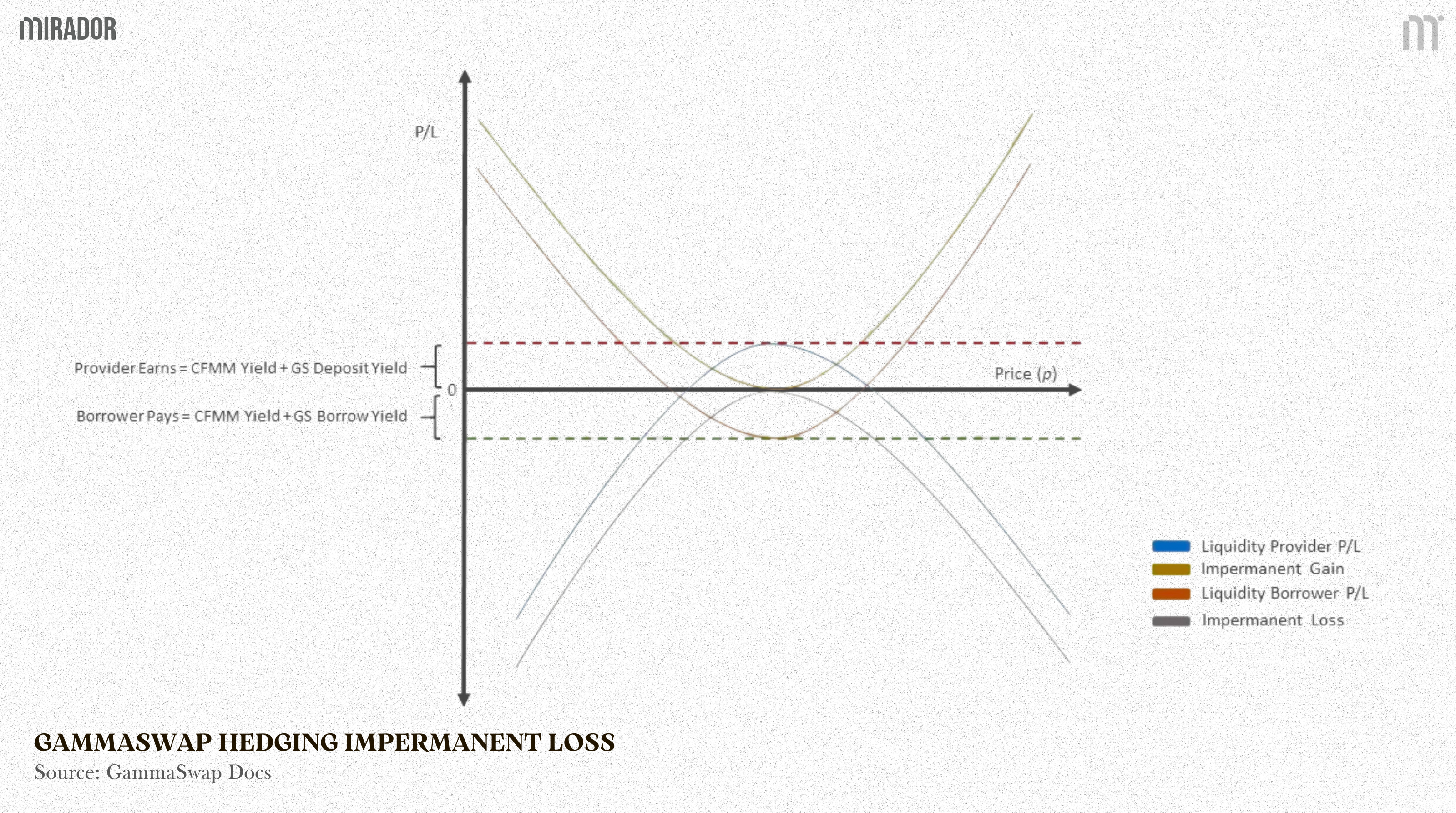
Referring back to the impermanent loss curve established in our previous analysis, we have:
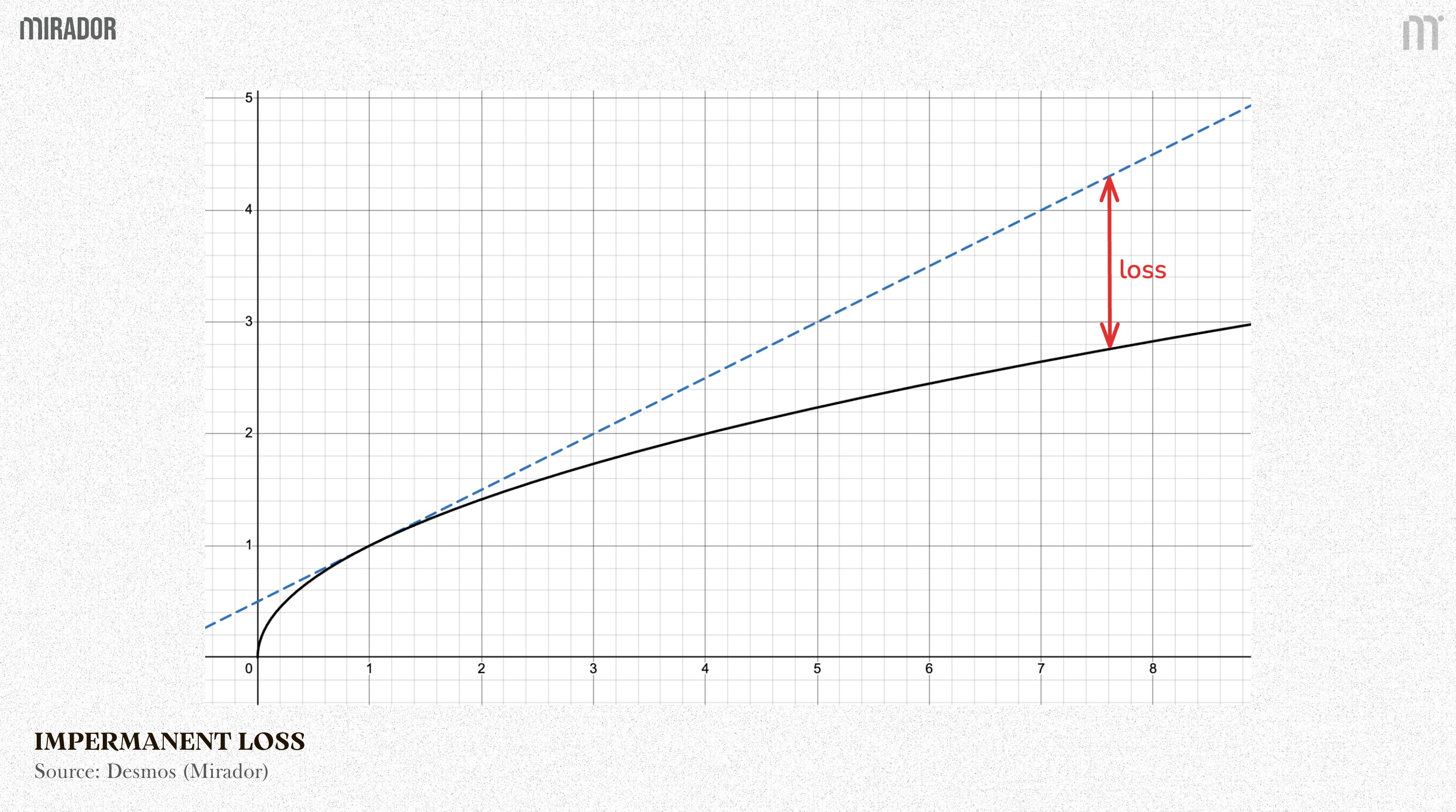
Blue dashed line (Holding a 50/50 portfolio): This represents the case where you do NOT provide liquidity. You simply hold 50% of one asset and 50% of the other in your wallet (for example, 50% ETH and 50% USDC).
Black solid line (LP value in a X*Y=K AMM): This represents the case where you provide liquidity to a standard AMM pool (such as Uniswap V2), which follows the X*Y=K formula.
(1) Observing how Delta changes
Let’s look at the solid black curve that represents the value of an LP position.
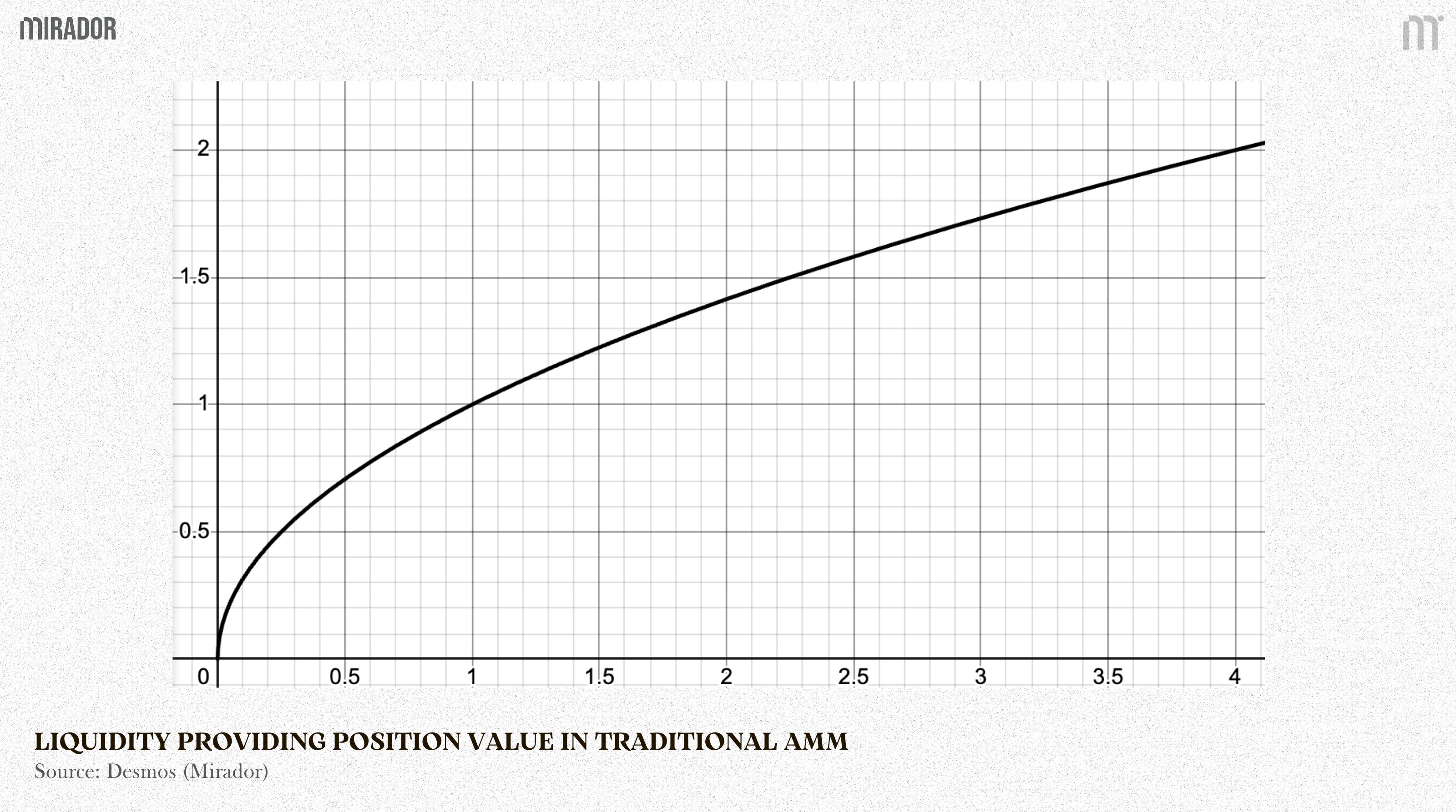
As price goes up (moving to the right on the x-axis): The black curve becomes flatter. Its slope decreases compared to the steep slope near the starting point.
This can be explained that: when price increases, AMM automatically sells part of the asset that is going up in order to keep the pool balanced. Because you now hold less of the increasing price asset, the growth of your portfolio slows down.
In other words, your delta decreases as price moves away from the starting point.
These come directly from the formula used to compute the value of a LP position in a constant-product AMM:
The value of the pool can be written as:
Taking the first derivative of V with respect to price P, we have delta:
From this expression, the intuition is immediate: since P appears in the denominator, delta decreases as price increases.
(2) From decreasing Delta to negative Gamma
As we have mentioned before, gamma measures how delta changes as price moves. At its core, gamma is simply the derivative of delta, simply written as:
Taking the derivative of delta with respect to P, we have:
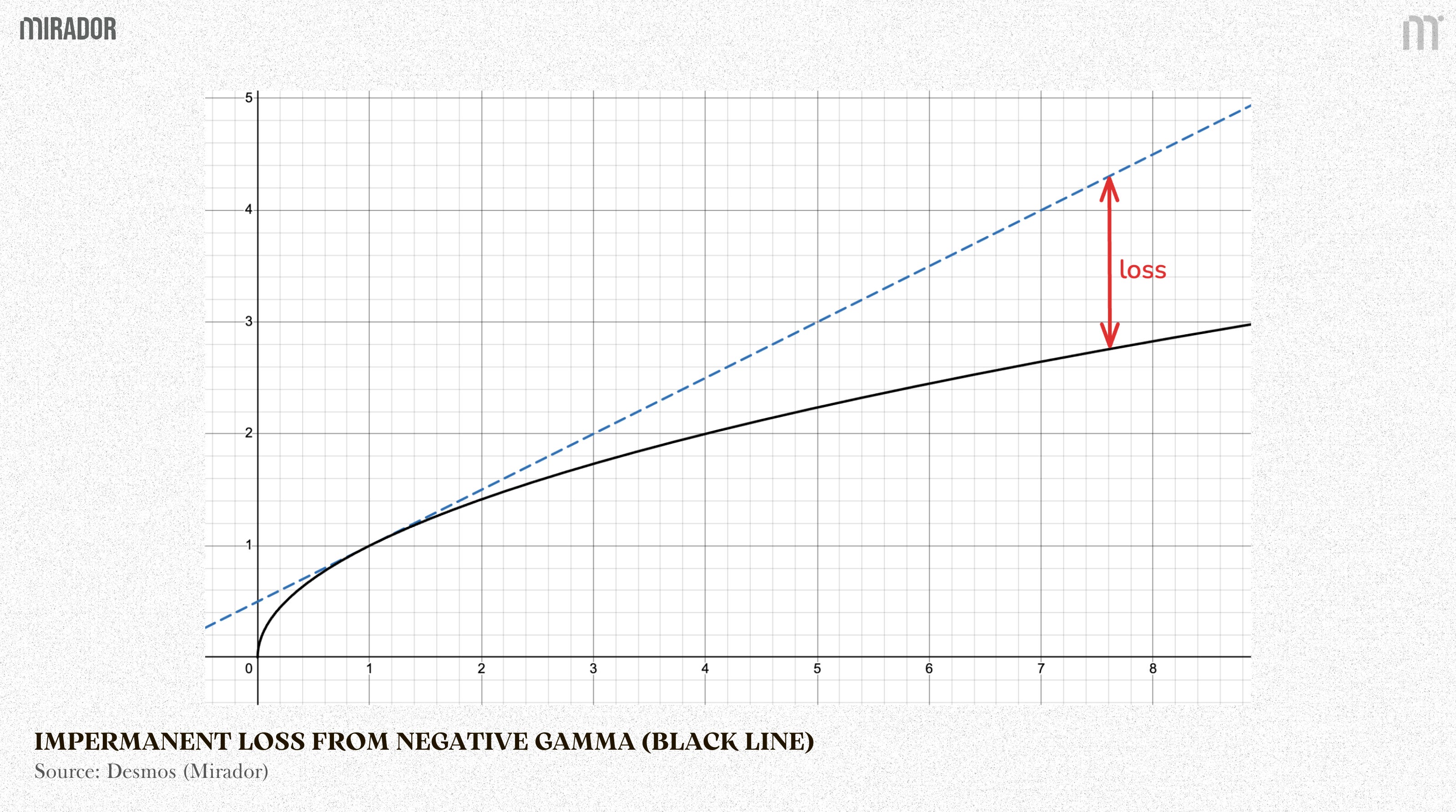
This result shows that anyone providing liquidity to a constant-product AMM (for example, Uniswap V2) is structurally exposed to negative gamma. The curvature of the LP payoff is an inherent consequence of the AMM design, not of market conditions or trading behavior.
Geometrically, negative gamma produces a downward-curving (concave) shape. This explains why the LP curve (black) always lies below the HODL curve (blue dashed line) as price moves further away from the initial level.
(3) Impermanent Loss
For comparison, consider the HODL position. Its value changes linearly with price, which means its delta is constant. Since delta does not change as price moves, its derivative with respect to price is zero. In other words, the HODL position has zero gamma.
Mathematically:
This contrast highlights the core difference between holding assets and providing liquidity. In other words, the red “loss” area on the chart is a direct consequence of negative gamma pulling delta down.
Therefore, no matter whether the price goes up or down, keeping your funds in a liquidity pool results in a lower total value than if you had just held the same assets in your own wallet. Moreover, this loss becomes increasingly pronounced as the asset price continues to rise.
————————————————————————————
This explains why swapping gamma for hedging purposes becomes necessary for liquidity providers. Once impermanent loss is understood as a direct consequence of negative gamma, it is clear that LPs are exposed to a form of risk they did not explicitly choose.
Viewed through this lens, GammaSwap went live in 2023 to address impermanent loss by allowing LPs to hedge their gamma exposure, using a financial instrument that is directly tied to gamma itself - options (perpetual options).
The next section will walk through perpetual options trading in GammaSwap and explain the concept of PnL when trading on it.
SECTION 3: GAMMASWAP – ONCHAIN PERPETUAL OPTION
Since options are the clearest type of derivative that having both zero and non-zero gamma, they are a natural way to swap gamma.
And to keep hedging continuous without having to roll positions, perpetual options (options with no expiration), are the most practical choice.
In this section, we do not go into a detailed breakdown of how GammaSwap perpetual trades work (this is covered in a previous article). Instead, the focus is on explaining how profits and losses arise when taking positions that are effectively bets on volatility, or gamma.
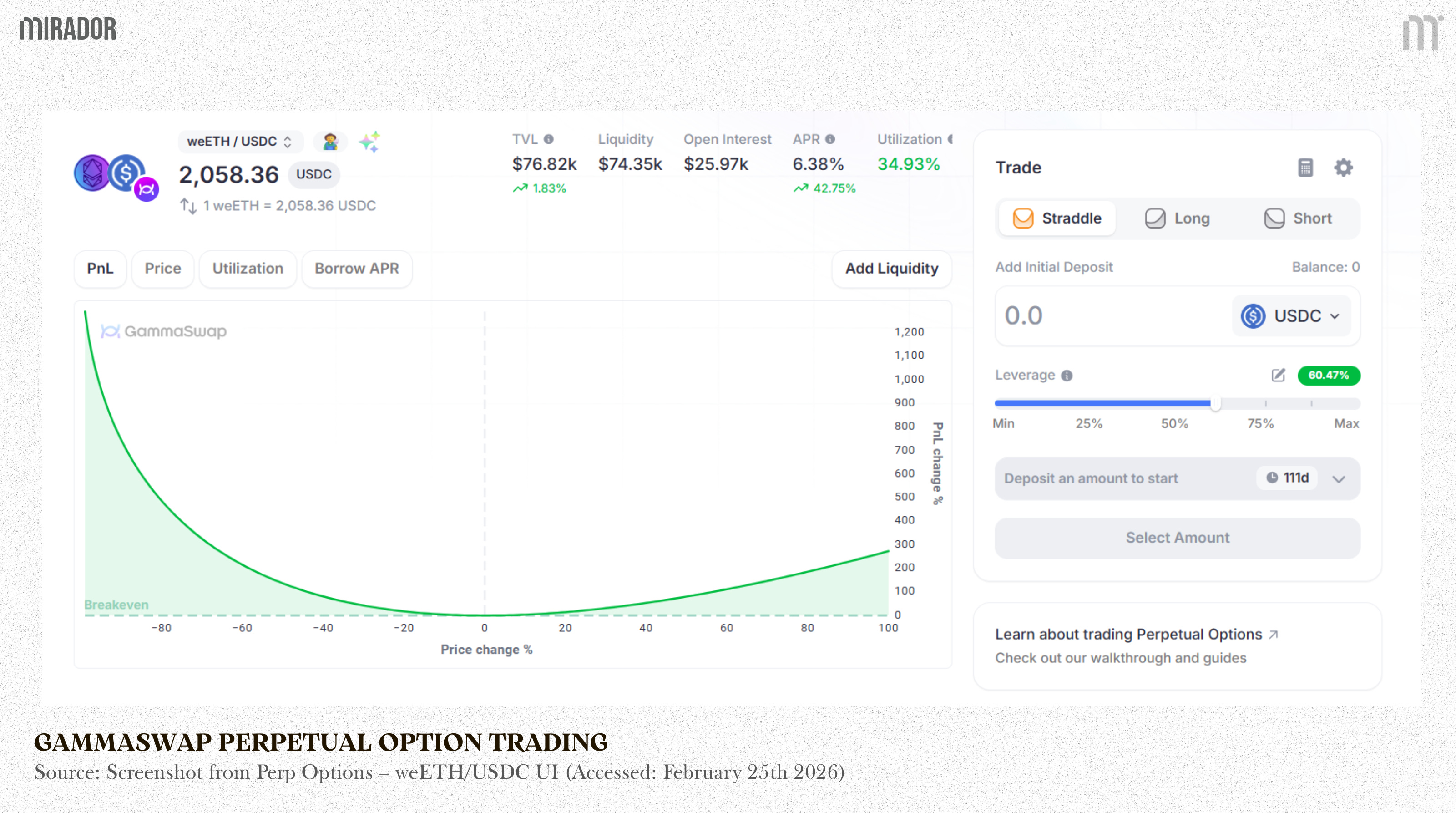
In essence, providing liquidity is economically similar to holding a short straddle option position, where you are short volatility and lose as price moves further away from its initial level.
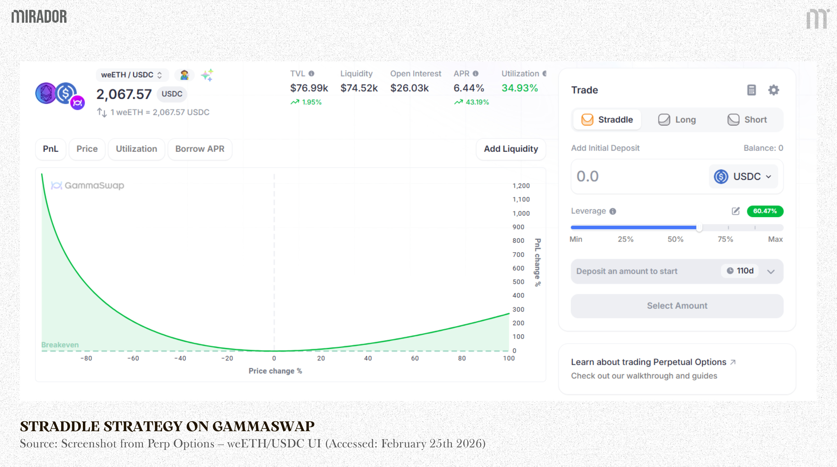
Straddle Position – Hedging Impermanent Loss
A straddle position is a borrowed LP position where the withdrawn collateral is split in a 50:50 ratio between the two tokens. This makes it the direct opposite of a standard LP position.
GammaSwap gives you the opposite exposure of a liquidity provider. When you open a perpetual option position (such as a straddle, long, or short), the protocol burns the LP token and locks the underlying assets in a smart contract. Your position is then tracked using the liquidity invariant, the same x⋅y=k relationship used by the contant-product AMM like Uniswap V2.

For example: Suppose Alice borrows $1,000 worth of ETH and USDC when ETH is priced at $2,000. This burns $1,000 of LP tokens and leaves them holding 0.25 ETH and 500 USDC in a perpetual option straddle.
The position follows the constant-product rule x⋅y=k, so here
Now assume ETH rises to $3,000, the new pool price implies:
Now solve the system:
We have result is x≈0.204
Then, after rebalancing, we have:
Meanwhile, the borrowed assets are no longer subject to AMM rebalancing, because the LP position is burned and the underlying assets are locked in the perpetual option contract rather than remaining inside the pool. Their value simply follows the market price:
0.25 ETH × 3,000 + 500 USDC = $1,250
As a result, the straddle owner holds collateral worth $1,250 while owing a debt worth $1,225, earning a profit of $25 (ignoring fees).
Therefore, “impermanent loss” here becomes “impermanent gain”.
The mechanism is essentially a swap: loss arises when an LP position underperforms HOLD position, while gain emerges when that same LP position is borrowed out and converted back into a HOLD exposure.
The swap-design we have mentioned above is enabled by the way that: Payoff on GammaSwap is created by flipping the LP’s position.
As a result, the trader moves from a payoff that curves downward (loses from volatility) to one that curves upward (profits from volatility). Paying a fixed cost in exchange for unlimited upside from price movement is exactly the defining feature of swapping gamma.
Although GammaSwap positions are fundamentally built on a straddle-like payoff (benefiting from volatility rather than pure direction), long and short positions introduce an important modification: directional rebalancing.
Instead of keeping the borrowed LP position neutral, the protocol intentionally rebalances the collateral toward one side.
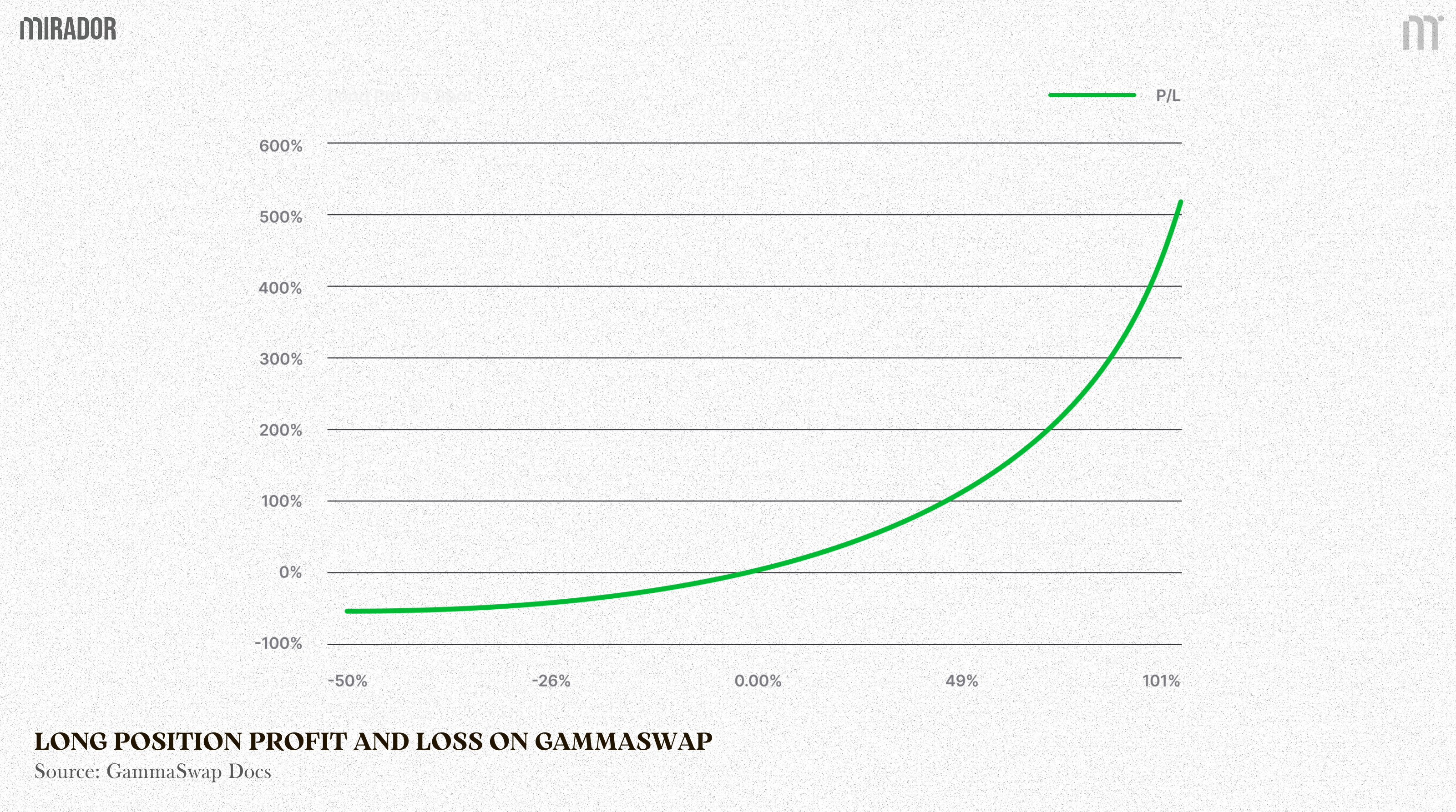
Long Position
In a long position, more weight is shifted toward the volatile asset (e.g. ETH), tilting the straddle upward and making it behave more like a call option.
For example, if a trader opens a $1,000 notional long position, 60% of the position will be in ETH ($600) and 40% of the position will be in USDC ($400).
At its core, this position remains a straddle, the PnL curve is still a convex, volatility-driven payoff, not a directional linear exposure like future.
What changes is not the structure, but the weighting.
By adjusting the token ratios, the trader intentionally introduces a directional bias. This reweighting tilts the payoff profile, making one side of the straddle more dominant and expressing a preferred direction, without abandoning the underlying long-volatility thesis.
In practice, even with directional bias, the position retains its convex PnL shape.
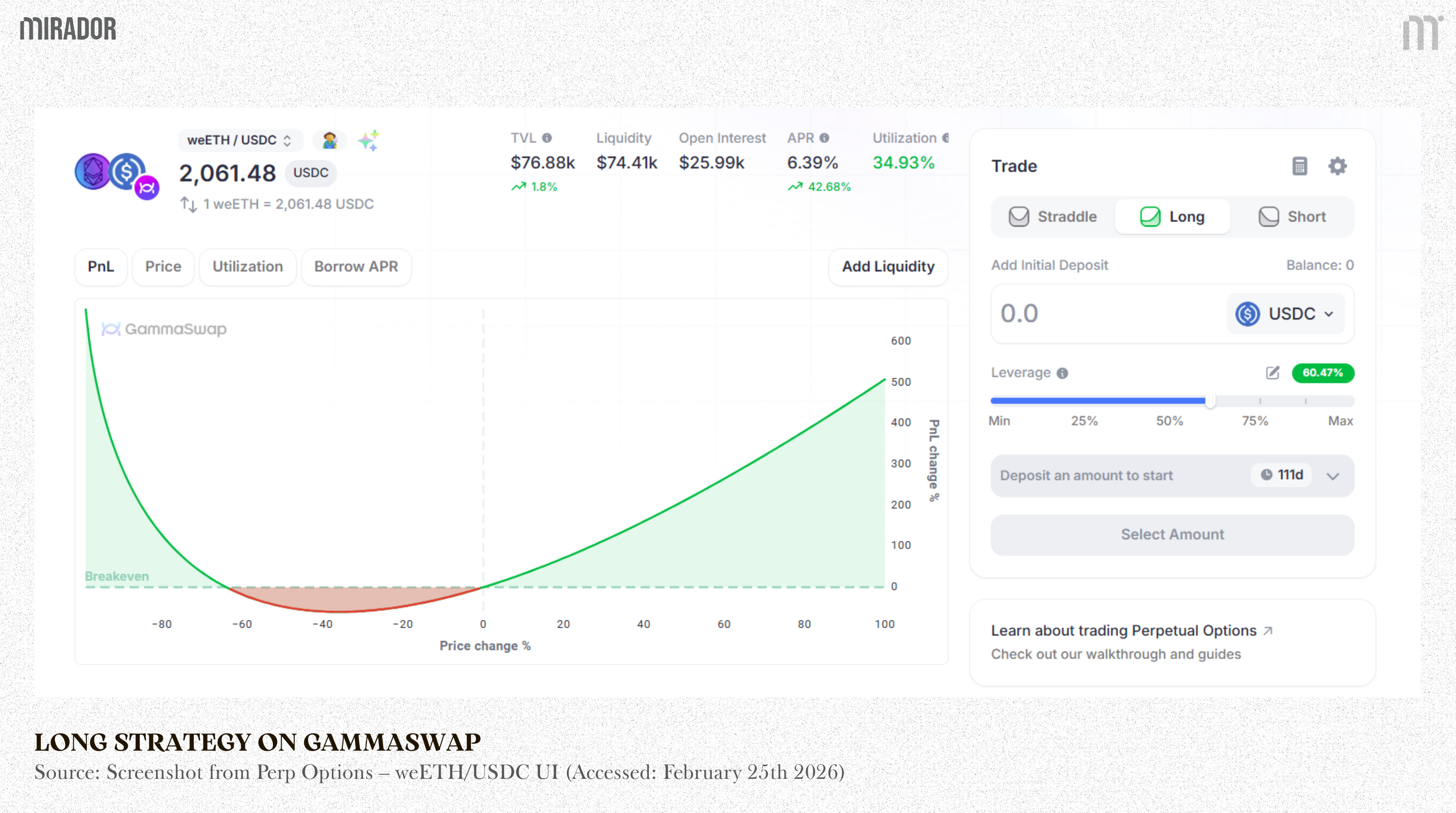
Therefore, a sufficiently large move in the opposite direction can still generate positive PnL, because a straddle profits from price displacement rather than direction.
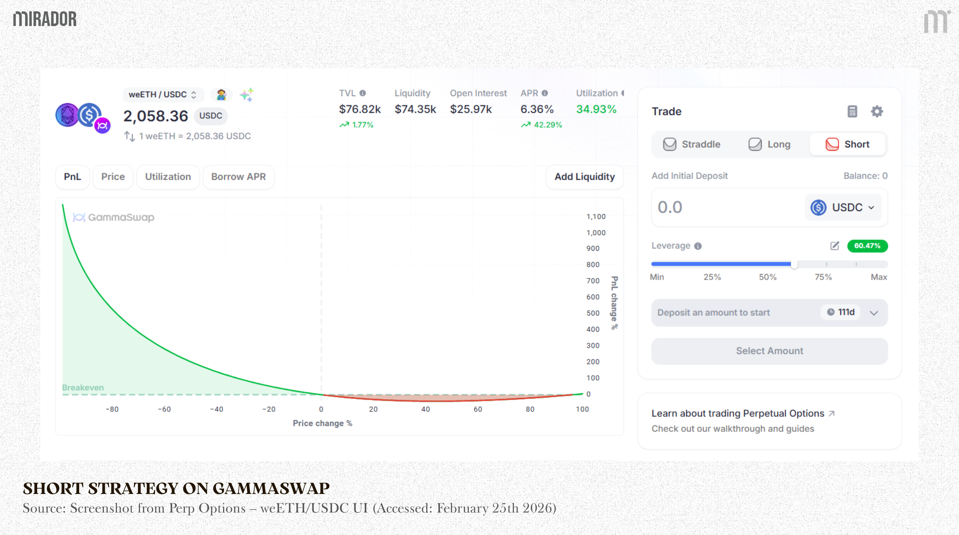
Short Position
In a short position, more weight is shifted toward the stable asset (e.g. USDC), tilting the straddle downward and making it resemble a put option.
For example, if a trader opens a $1,000 notional short position, 40% of the position will be in ETH ($400) and 60% of the position will be in USDC ($600).
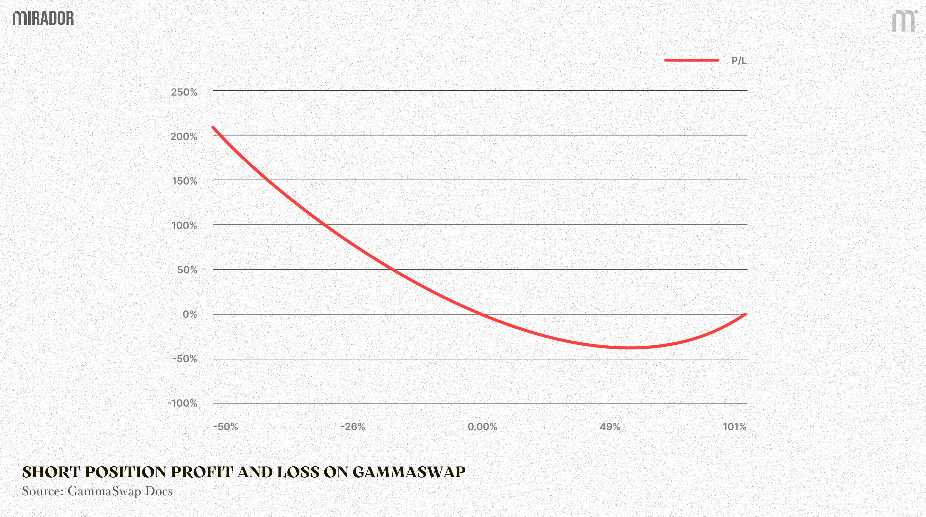
Crucially, this does not turn the position into a linear future. The payoff remains convex, and delta is still dynamic. The rebalancing simply biases the straddle so that as price moves, exposure naturally leans toward the winning side: ETH when price rises, or USDC when price falls, while still retaining the gamma-driven nature of the position.
Position PnL in practice due to AMM volatility
Across all three strategies, the PnL generated during downside price moves is consistently higher than that from equivalent upside moves.
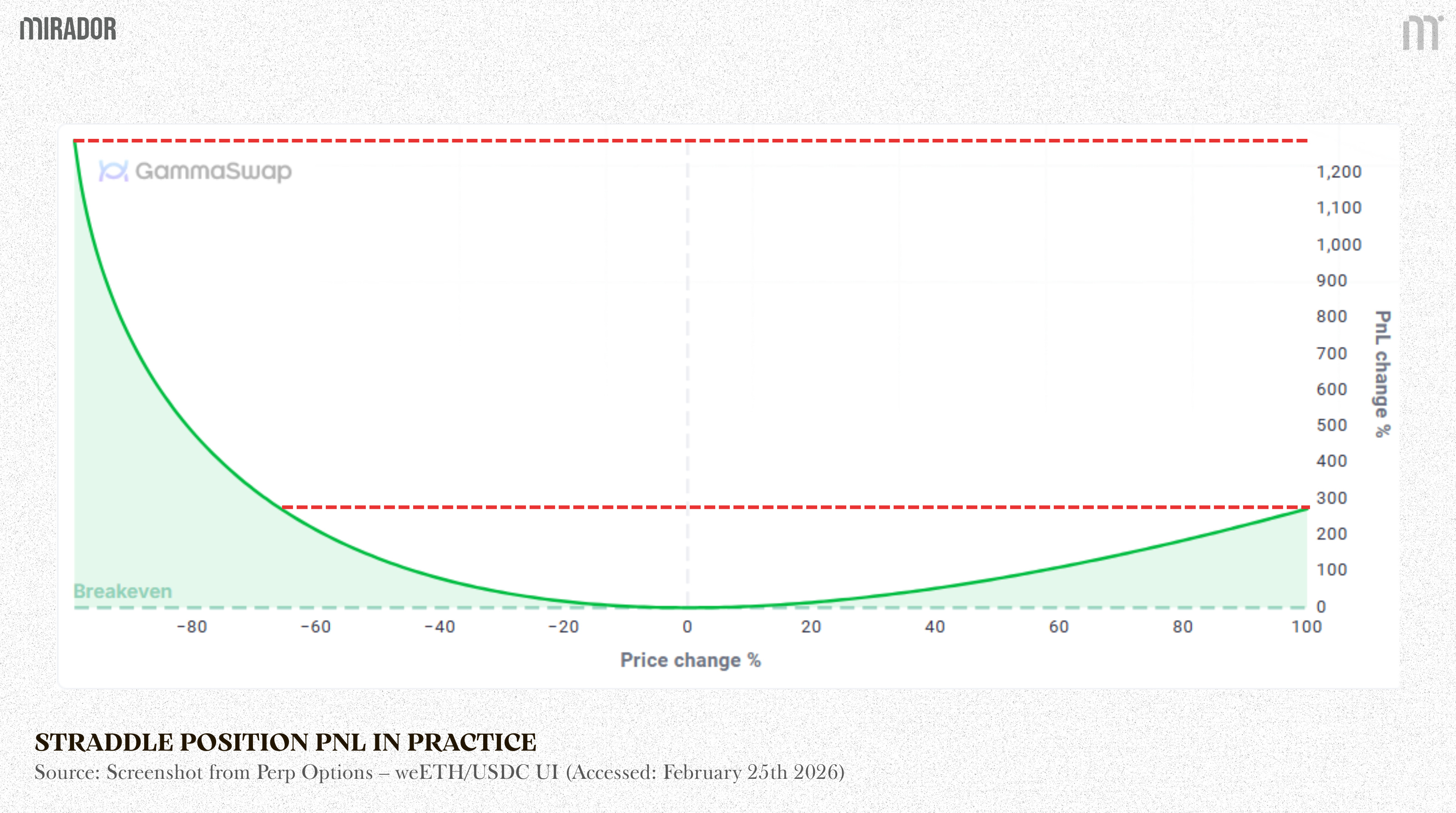
Straddle PnL
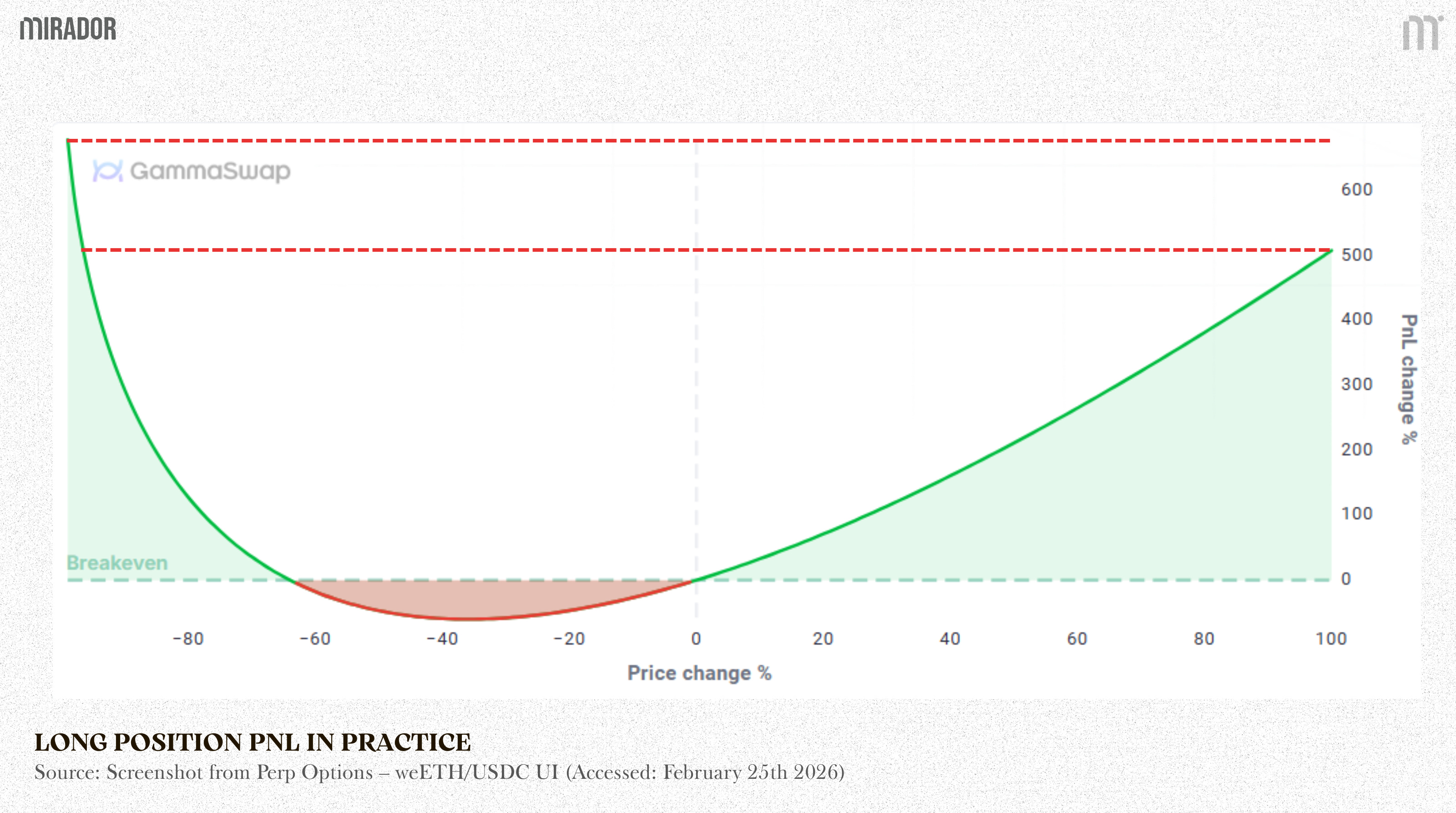
Long PnL
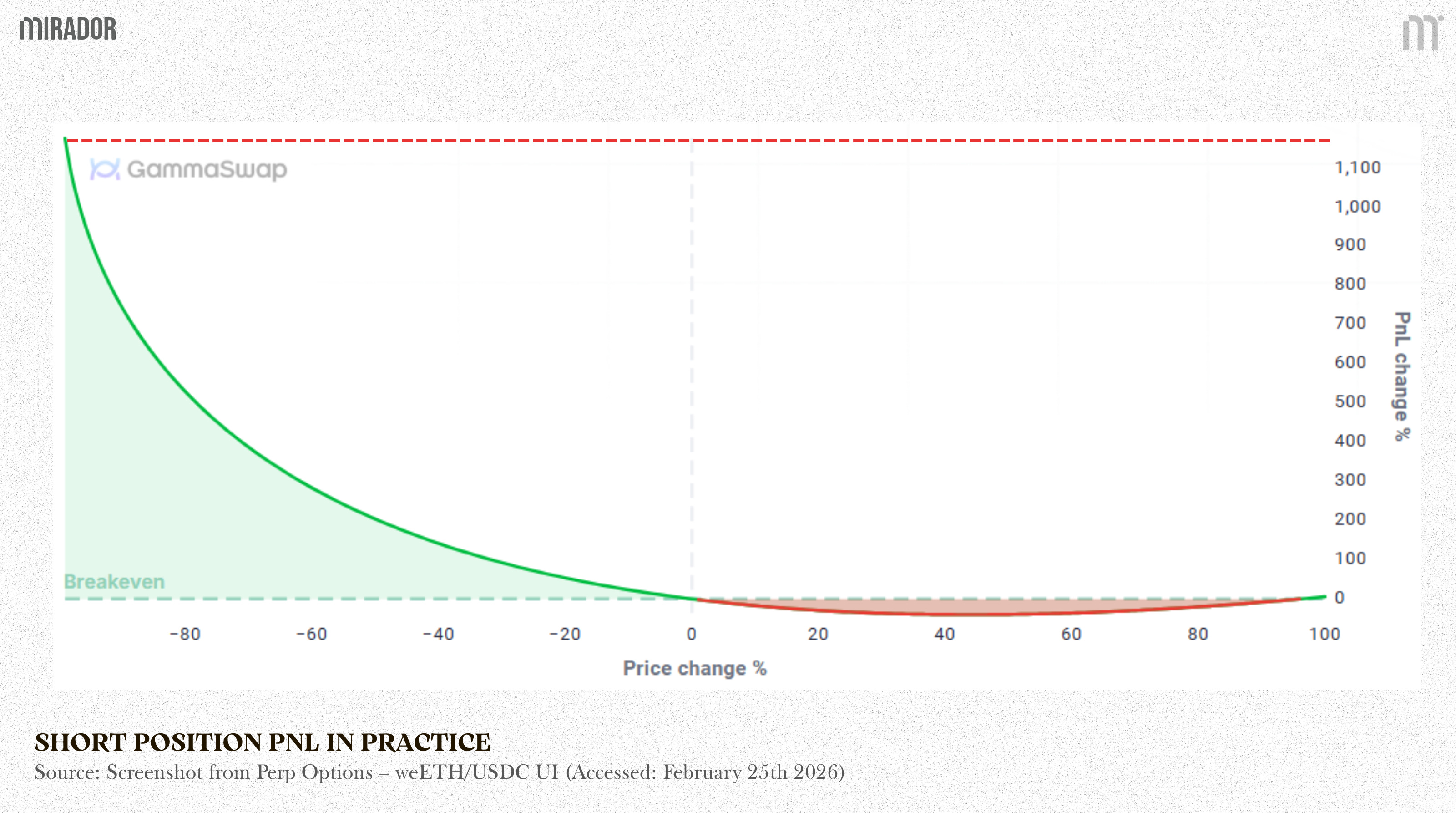
Short PnL
In theory, a straddle produces a symmetric, convex payoff: gains increase as price moves away from the entry in either direction.
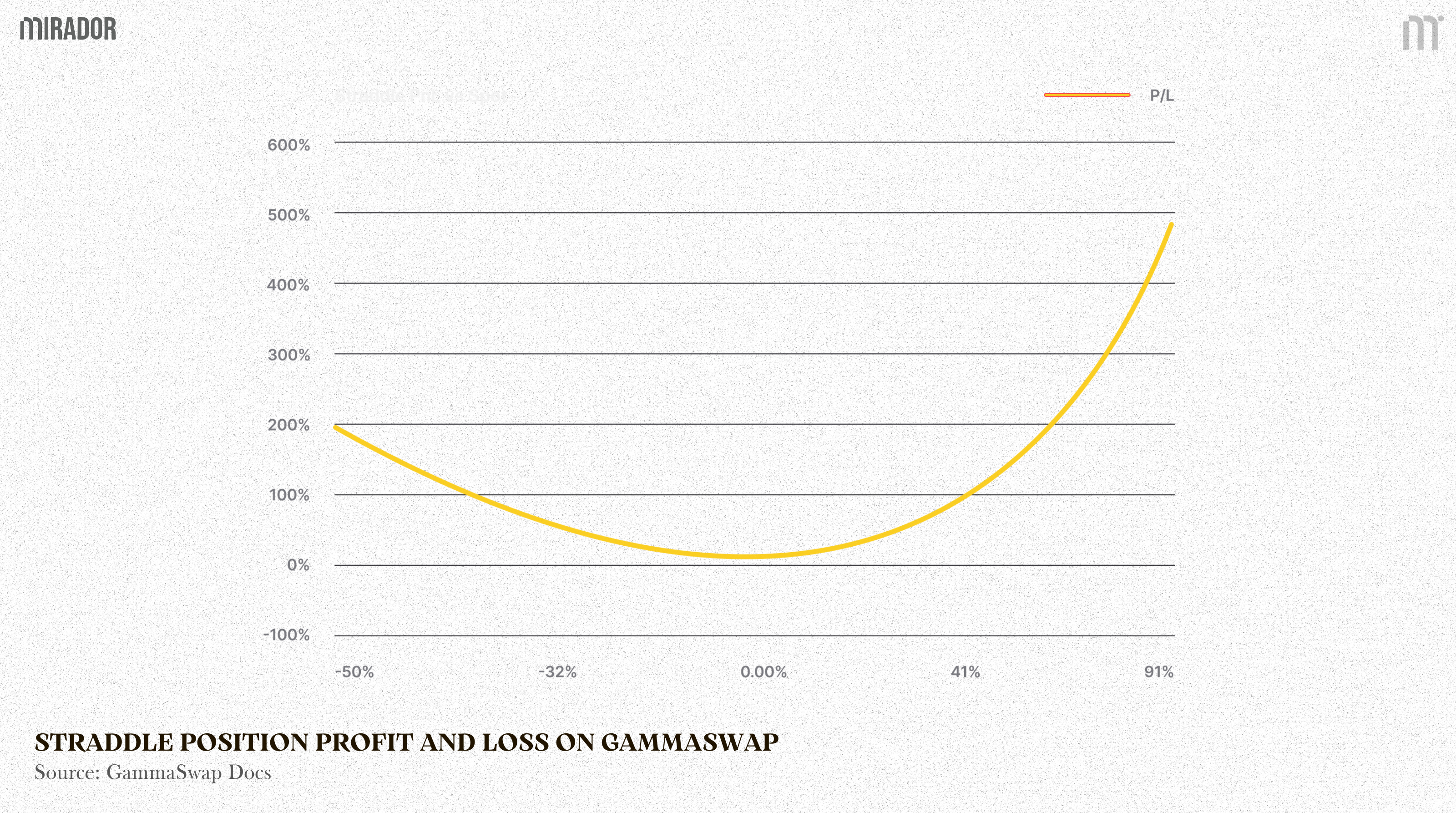
The theoretical PnL of a straddle forms a smile-shaped curve. As the price moves away from the strike in either direction, the payoff rises symmetrically.
In options theory, this shape is commonly referred to a smile shape.
This smile reflects the idea that position’s PnL increases as the market price moves deeper into OTM or ITM regions relative to the strike.
However, real markets rarely behave in such a balanced way. In practice, the smile is often distorted into a skew, where PnL rises more on decrease side of the price distribution than the other.
In GammaSwap, the notion of delta differs fundamentally from that of traditional options. Delta does not arise from a predefined option payoff, but is endogenously generated by the AMM liquidity formula itself.
As the underlying price moves, the pool’s inventory composition changes mechanically, resulting in a price-dependent delta exposure of the position:
With:
S is the current price,
K is the strike price
L is the liquidity constant (a variable set by protocol)
Therefore, we have:
When price falls (S→0 ): The term 1/√S, grows very fast. As a result, delta changes sharply, making the left side of the PnL curve rise much more steeply.
When price rises (S→∞): The term 1/√S slowly moves toward zero. Delta approaches a constant value 1/√K, so the right side of the PnL curve still increases, but in a smoother and more controlled way.
For the same percentage price move, downside moves cause delta to change much more than upside moves. This mathematical asymmetry is why GammaSwap PnL curves are naturally skewed and much steeper on the left side.
Because delta accelerates rapidly as price falls, a long volatility position effectively turns into a strong short position the moment the market starts to panic.
This means you profit significantly more from a 20% price drop (for example) than from a 20% price increase. This makes GammaSwap an especially powerful hedging tool for portfolios that are heavily exposed to spot tokens.
CONCLUSION
Impermanent loss is not simply an unavoidable cost of DeFi liquidity provision, but as a direct consequence of negative gamma exposure embedded in AMM design. By analyzing liquidity pools through the lens of options theory, we see that providing liquidity is economically equivalent to selling volatility, a short straddle position with fixed gamma and adverse convexity.
GammaSwap introduces a new on-chain primitive: perpetual options built from liquidity borrowing, allowing this gamma exposure to be explicitly transferred, hedged, or traded.
DISCLAIMER:
This article serves as a conceptual foundation for understanding GammaSwap.
Our focus here is not on the operational details of the protocol, but on the idea of “gamma swapping” from first principles, connecting options theory with impermanent loss in AMM mechanics. We aim to help readers clearly understand the structural logic behind impermanent loss, negative gamma exposure, and how perpetual options can be used to reshape that risk.
We do not avoid formulas or mathematical reasoning, but everything is simplified and presented step by step so that the core intuition becomes clear.
In the next article, we will move from theory to mechanism, breaking down step by step how GammaSwap structurally flips negative gamma exposure and turns “impermanent loss” into what can become “impermanent gain.”