IMPERMANENT LOSS AND HOW YIELDBASIS MAKES IT “ZERO" - PART I: IMPERMANENT LOSS - A SIMPLE MATHEMATICAL EXPLANATION

Jan 22, 2026

INTRODUCTION

Impermanent loss is one of the most confusing concepts in DeFi. Many people hear the term, experience the result, but never fully understand where it comes from and whether LP trading fee can cover this loss.

In part I of this series, we take a step back and look at impermanent loss from its mathematical roots. From there, we explain why Yield Basis uses a carefully designed 2× leveraged structure to neutralize this effect and how protocols keeps this leverage overtime.

KEY TAKEAWAYS

This part I explains impermanent loss from first principles and shows how Yield Basis redesigns the payoff structure to eliminate it at the source.

Section 1: Explaining how impermanent loss naturally arises from traditional AMMs and examining the coverage ability of tradining fee.
Section 2: The basis of YieldBasis innovation to solve impermanent loss at its core

In traditional finance, idle capital usually leads to two familiar choices: speculation (such as buying gold and waiting for price appreciation) or earning yield by depositing it in a bank.

Crypto follows the same logic. With idle tokens, you generally choose between:

(1) Holding them to gain from price movements or

(2) Providing liquidity to earn trading fees.

This trade-off causes opportunity cost, it is also where impermanent loss comes in.

SECTION 1: IMPERMANENT LOSS – A RESULT OF BONDING CURVE

Impermanent loss doesn’t mean you lose tokens. In practice, it represents the opportunity cost of providing liquidity: When prices move, the AMM of liquidity pool automatically rebalances your position. This rebalancing can leave your liquidity position worth less than if you had just held the assets outside the pool. That gap is what we call impermanent loss.

To better understand how “your liquidity position worth less than if you had just held the assets outside the pool”, we start by building a graph that compares two strategies: holding assets versus providing liquidity, over different price levels

The x-axis represents the price change of the asset (for example: BTC) relative to the starting point

$x = \frac{\text{New BTC value}}{\text{Initial BTC value}}$

The y-axis represents the position’s total value change, showing how much the position is worth relative to the starting point

$y = \frac{\text{New total value of position}}{\text{Initial total value of position}} = \frac{V_{new}}{V_{initial}}$

Each strategy gives different relationship of x and y.

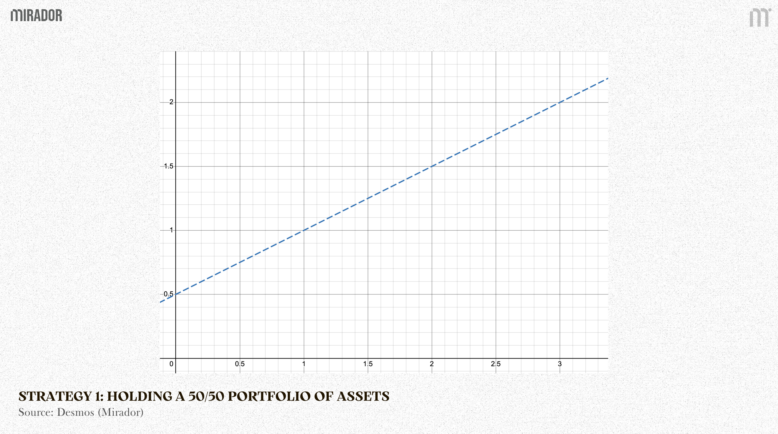
Strategy 1: Just holding a 50/50 portfolio of assets (for example: BTC and USDC)

This strategy means initially, the total value of BTC holding is equal to the total value of USDC (50:50 ratio).

Therefore, initial total value of portfolio (V_initial) is defined:

$V_{initial} = 0.5 \times V_{BTC, initial} + 0.5 \times V_{USDC, initial}$

$0.5 \times V_{BTC, initial} = 0.5 \times V_{initial}$

Suppose that BTC price increase x times, we have new total value of portfolio (V_new) is:

$V_{new} = 0.5 \times V_{BTC, new} + 0.5 \times V_{USDC, new}$

since USDC stay the same, we have

$V_{new} = 0.5 \times V_{BTC, new} + 0.5 \times V_{initial} $

$V_{new} = (0.5 \times V_{BTC, initial}) \times x + 0.5 \times V_{initial}$

$V_{new} = 0.5 V_{initial} \times x + 0.5 \times V_{initial}$

Therefore:

$x = \frac{V_{new} - 0.5 \times V_{initial}}{0.5 \times V_{initial}}$

Because

$y = \frac{\textit{New total value of position}}{\textit{Initial total value of position}} = \frac{V_{new}}{V_{initial}},$

after transformation, we have

$x = \frac{(y - 0.5) \times V_{initial}}{0.5 \times V_{initial}}$

$y = 0.5x + 0.5$

(linear line)

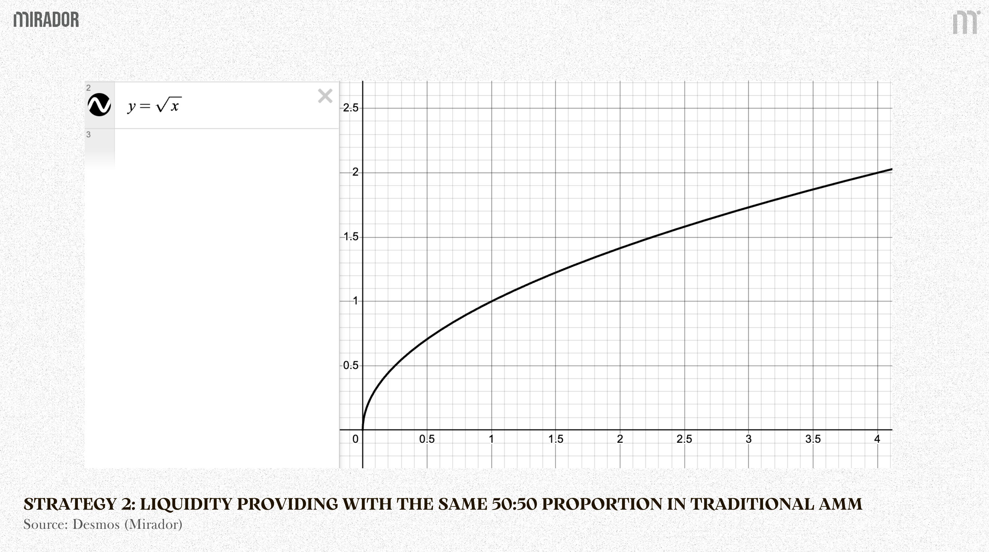
Strategy 2: Liquidity providing with the same 50:50 proportion (for example: BTC and USDC) in traditional AMM X*Y=K.

Important note: In the formulas below, we deliberately exclude trading fees, incentives, and rewards. This is done to isolate the pure effect of AMM rebalancing and price movement. Fees and incentives vary across protocols and market conditions, and including them would obscure the core mechanism behind impermanent loss.

Consider a constant-product AMM with:

A = quantity of BTC in the pool
B = quantity of USDC in the pool

The AMM enforces the invariant:

Therefore,

$B = \frac{K}{A} (1)$

BTC Price in terms of USDC =

Then:

$B = \text{BTC Price} \times A \quad (2)$

From (1) and (2), we have:

$\text{B}^2 = \text{BTC Price} \times A \times \frac{K}{A} = \text{BTC Price} \times K$

$B = \sqrt{\text{BTC Price} \times k}$

The total value of the liquidity position (V) is the sum of the BTC and USDC components:

$V = \text{BTC Price} \times A + B$

Replace (2), we have:

$V = 2 \times B = 2 \sqrt{\text{BTC Price} \times k}$

When asset price increases x times:

$V_{new} = 2\sqrt{\text{BTC Price} \times x \times k} = V_{initial} \times \sqrt{x}$

Therefore,

$y = \frac{V_{new}}{V_{initial}} = \frac{V_{initial} \times \sqrt{x}}{V_{initial}} \Leftrightarrow \mathbf{y = \sqrt{x}}$

(curve)

Now, let’s perform both strategy on the same graph:

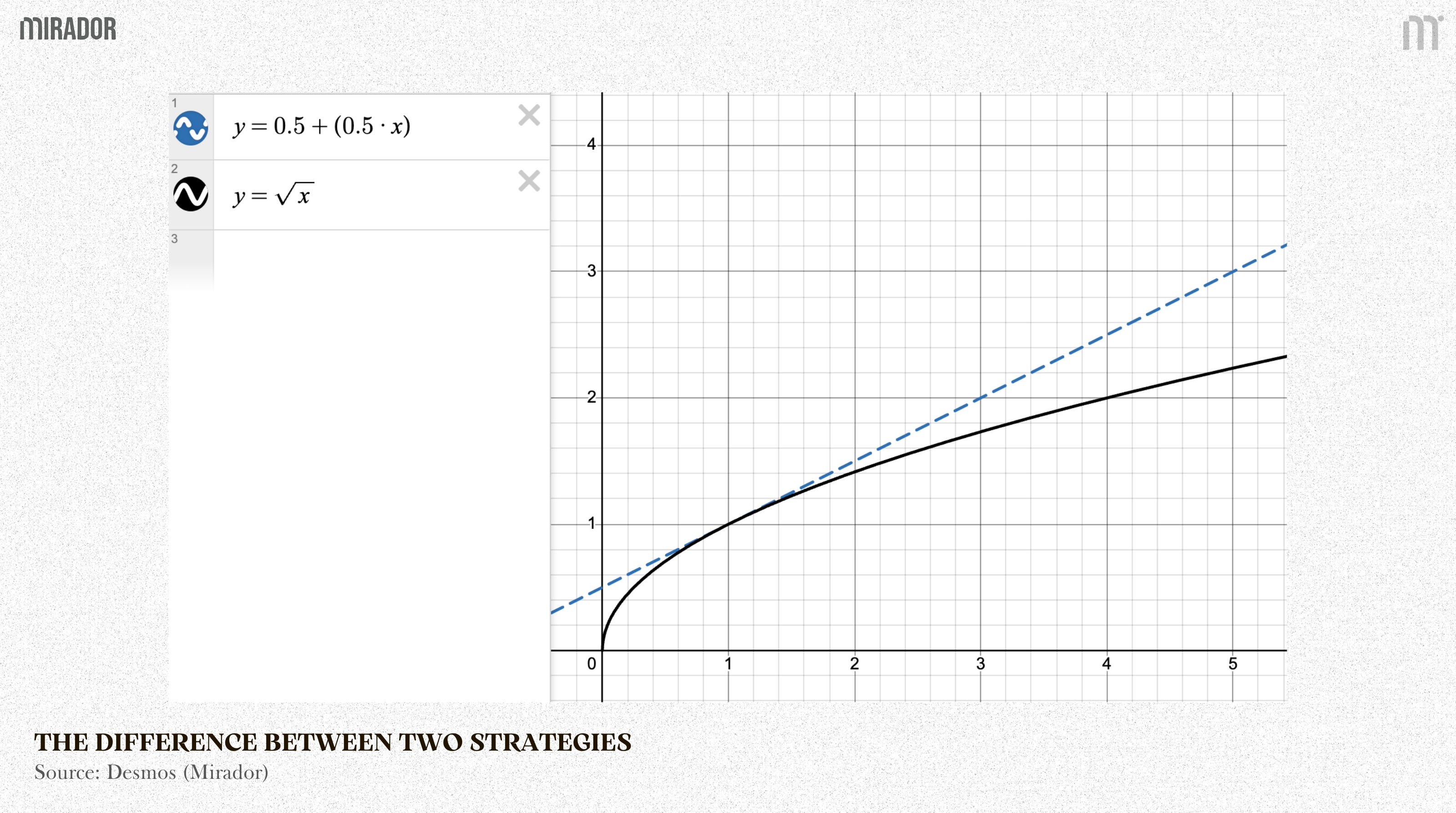
Blue dashed line (Holding a 50/50 portfolio): This represents the case where you do NOT provide liquidity. You simply hold 50% of one asset and 50% of the other in your wallet (for example, 50% WBTC and 50% USDC).
This line is linear (for example, if the price of $BTC doubles, the value of your $BTC portion also doubles). It’s very straightforward and intuitive.
Black solid line (LP value in a X*Y=K AMM): This represents the case where you provide liquidity to a standard AMM pool (such as Uniswap V2), which follows the X*Y=K formula.
This line is curved (it follows a square-root shape).

Then, it’s time to consider the “difference” between the black line and the blue dashed line. Theoretically, this difference can be either a loss or a gain, depending on how the two lines are positioned relative to each other.

To examine the difference between the two curves, we can apply the AM–GM inequality, which can be simply written as:

$\frac{a+b}{2} \geq \sqrt{ab}, \text{ for } a,b \geq 0.$

With a=x (x is price ratio so x ≥ 0 under all conditions), b=1, we have:

$\frac{x+1}{2} \geq \sqrt{x}$

<=>

$\Leftrightarrow 0.5x + 0.5 \geq \sqrt{x}$

This means that the black line (LP) always stays below the blue dashed line (HODL) as the price moves further away from the starting point. The difference, therefore, turns into the impermanent loss that we have mentioned before.

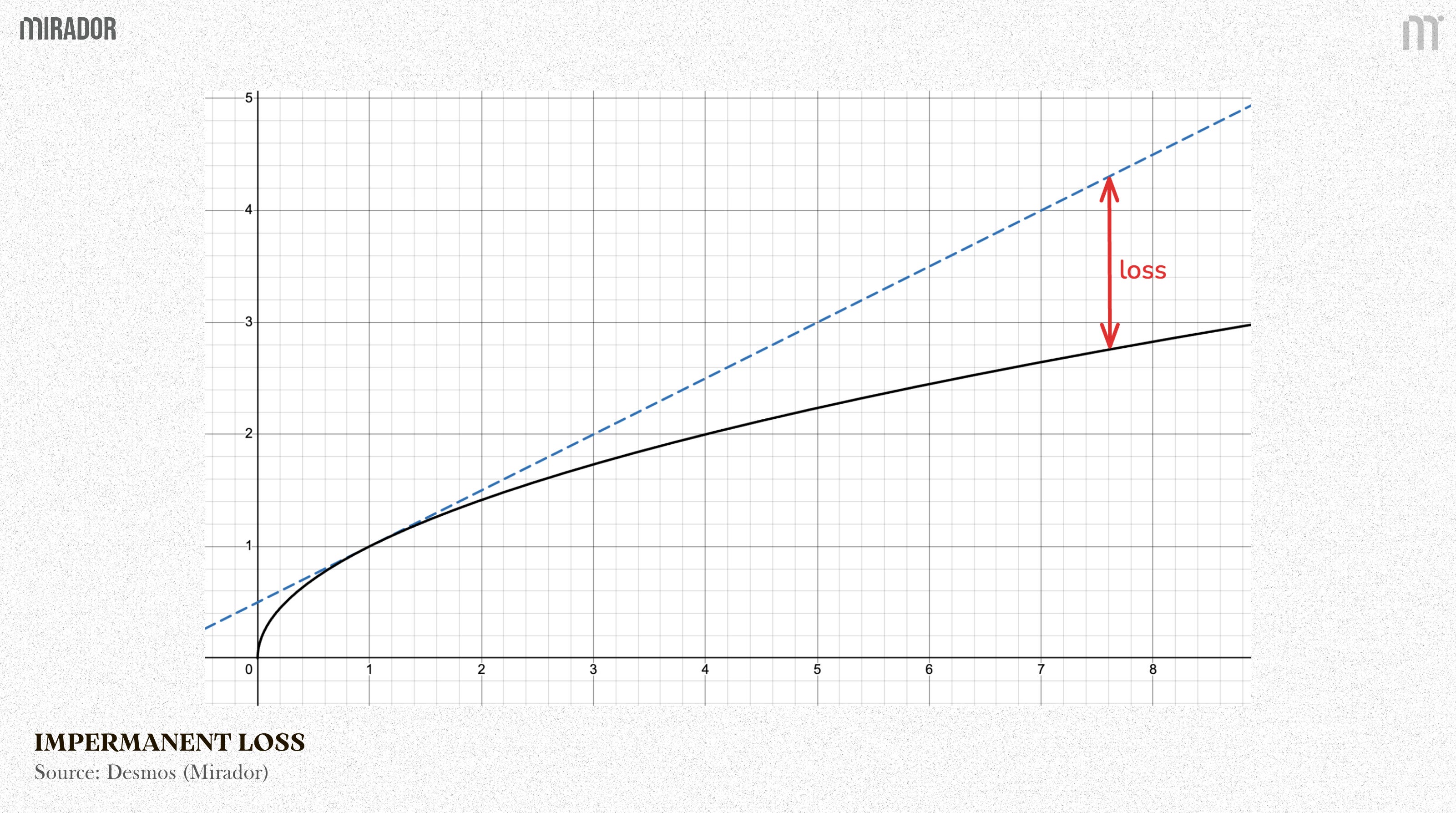
No matter whether the price goes up or down, keeping your funds in a liquidity pool results in a lower total value than if you had just held the same assets in your own wallet. Moreover, this loss becomes increasingly pronounced as the asset price continues to rise.

This gap is exactly what we call Impermanent Loss, and essentially, it should be understand as the opportunity cost due to selling assets too early. The main cause of it is the automatic rebalancing mechanism – the core concept of AMM.

Core concept: In a classic AMM, the core formula is:

Amount of Token A (x) × Amount of Token B (y) = Constant (k)

Assume you have a liquidity pool made up of BTC and USDC. The automatic rebalancing mechanism always tries to keep the total value of BTC in the pool equal to the total value of USDC (50:50 ratio).

When BTC’s price on the open market increases, the BTC price inside the AMM pool is temporarily lower.

This creates an arbitrage opportunity: Traders notice that BTC in your pool is cheaper than the market price, so they step in, sell USDC for your pool, buy BTC at that a lower price, and sell it elsewhere for a profit.

Therefore, the pool’s balance changes: number of BTC goes down, and number of USDC goes up, while their value is equal.

Similarly, whenever the price of either token in the pool goes up or down, new arbitrage opportunities are created. These arbitrage trades are exactly how the AMM continuously rebalances the pool, without the need for an order book or any intermediary.

The problem is: An AMM does not wait until the price reaches the top to sell. Instead, it sells gradually at every price step as the price goes up. That is exactly why LPs can never achieve the maximum profit compared to simply holding the asset and selling it at the peak.

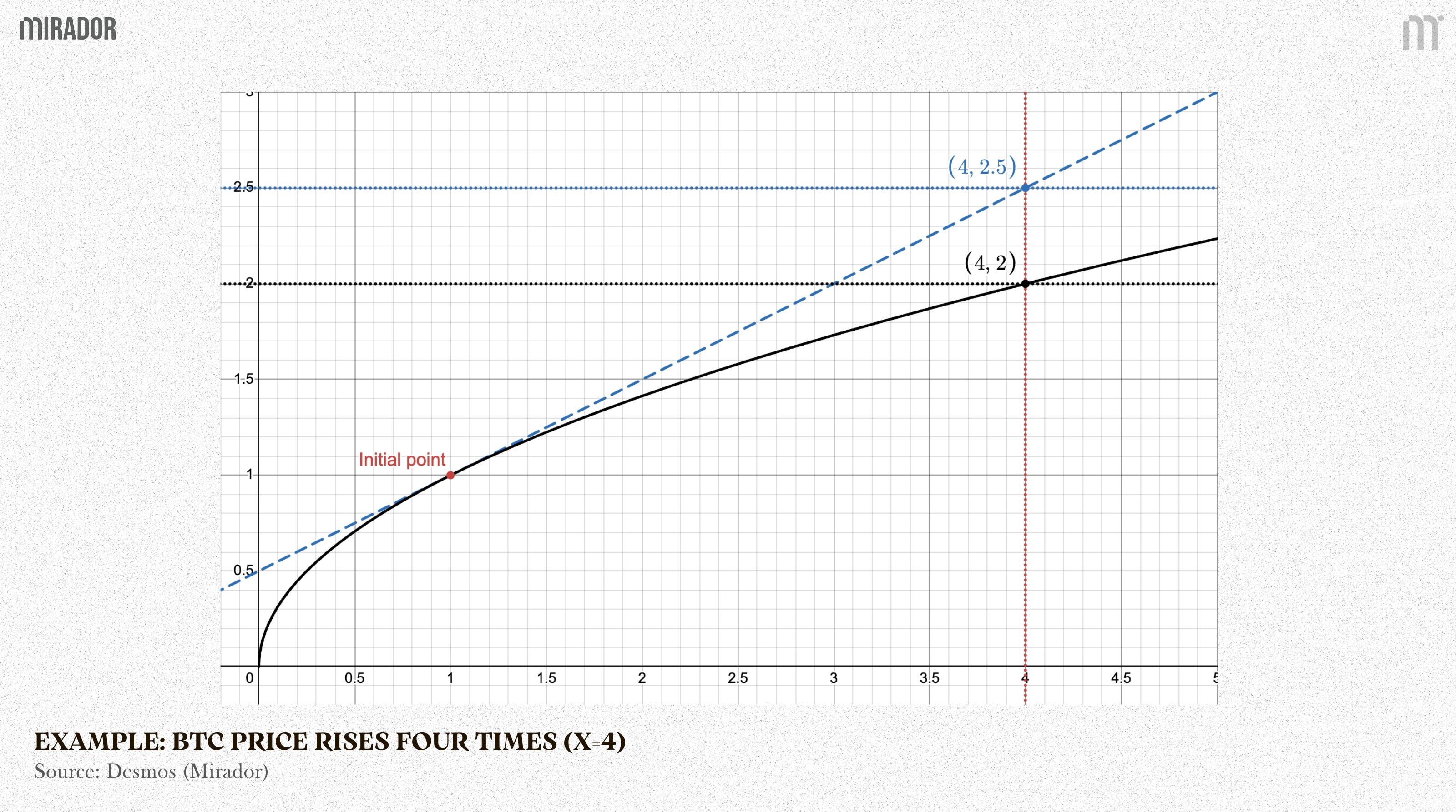
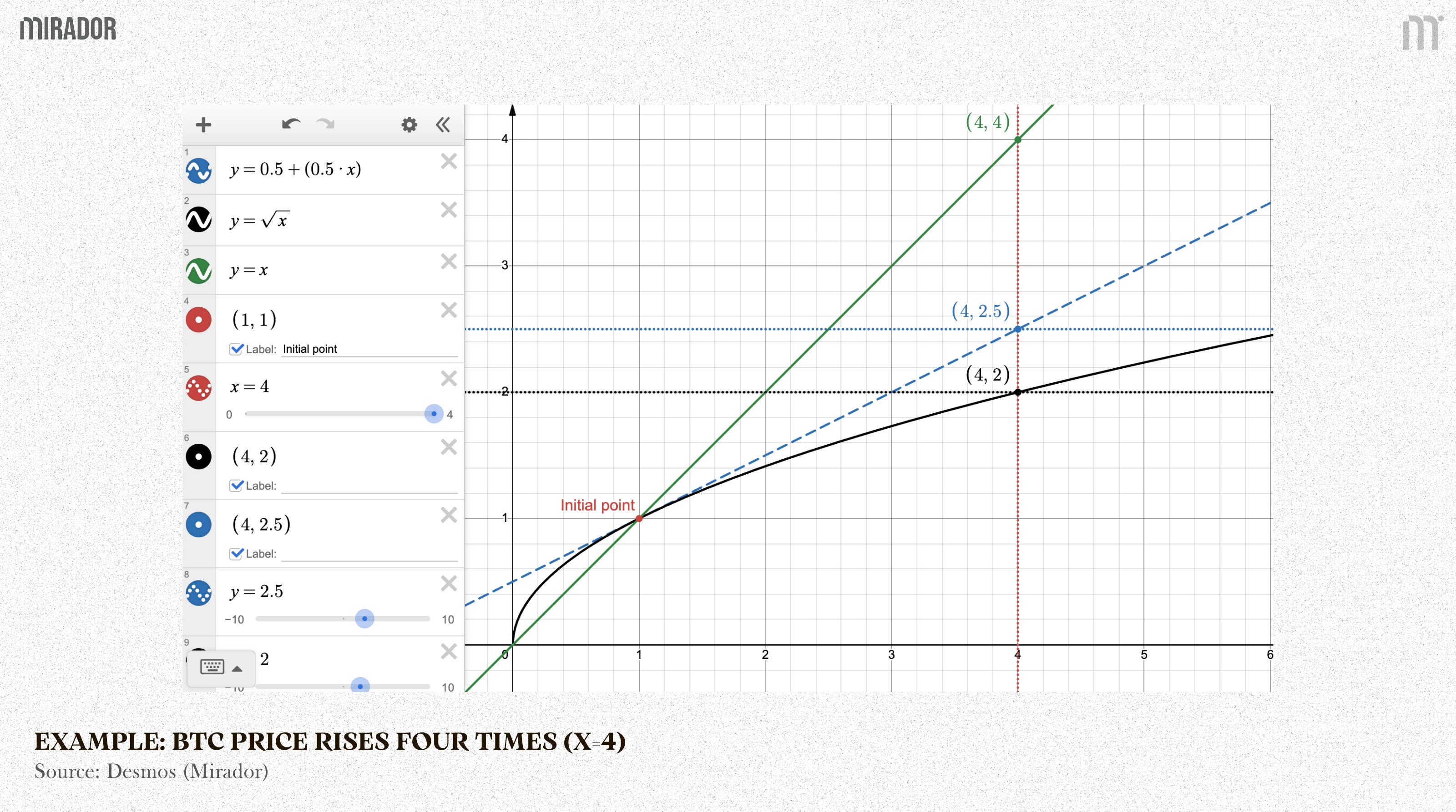
For example: You start providing liquidity in an AMM pool at the BTC price of $10,000. After a period of time, BTC price rises four times to $40,000 (x=4). Considering the same amount of BTC and USDC at the initial point, this increase in BTC price causes:

50/50 holding portfolio increases 2.5 times
LP position increases 2 times only.

Theoretically, AMM liquidity providers earn trading fees from pool activity. In reality, liquidity provision is most attractive in stable market environments, where fees are sufficient to offset impermanent loss and generate positive returns.

Whether trading fees can make up for impermanent loss depends on how much prices move and how much trading happens in the pool at a given time. Many studies have looked at whether trading fees can cover impermanent loss for liquidity providers, and most of them test this by running repeated simulations.

In this article, we build a simple assumption-based model that estimates the daily performance of being an LP of $5000 WBTC and $5000 USDC in the Uniswap v2 WBTC/USDC pool over two years, compared to simply holding the same 50/50 WBTC–USDC portfolio.

With

Price move metric (x): each day it takes the WBTC price in USD and computes

meaning how many times WBTC has moved versus the start date.

TVL: for each day, it takes the latest pool reserves before the day ends and converts them to USD to get TVL/day. TVL is a “stock” number (what’s in the pool at a point in time), and it’s used as the denominator for fee yield.
Volume (pool-level, from Swap events): for each day, it sums all swaps that actually happened inside this specific pool using the pool’s own Swap events.
Daily fee yield: it estimates daily LP fees as %fee/day = 0.3% × (volume / TVL) (0.3% is Uniswap v2’s fee rate). Fees are then accumulated using compounding.
Impermanent loss: with a price move , Uniswap v2’s no-fee LP value scales like , while a 50/50 hold scales like . So:

$\mathbf{IL} = \sqrt{x} - (\mathbf{0.5x + 0.5}).$

So , the model’s final comparison is

$\mathbf{net} = (\sqrt{x} \times \mathbf{fee\_factor}) - (\mathbf{0.5x + 0.5})$

If net < 0, estimated fees don’t offset estimated IL; if net > 0, they do.

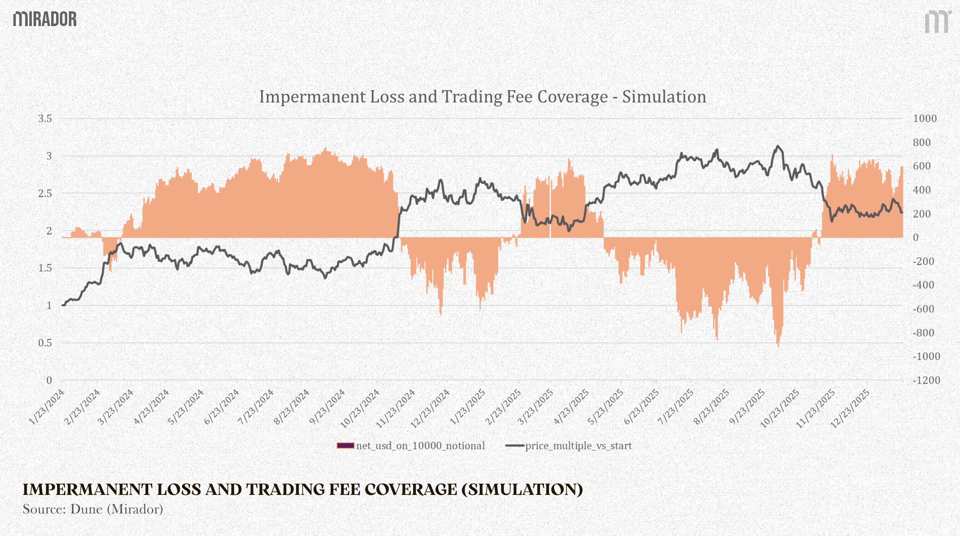
In this test case, we can see that as the volatility factor x increases (meaning the BTC price rises further from the starting point), trading fees become less effective at covering impermanent loss, and the resulting loss grows larger.

SECTION 2: HOW TO SOLVE IMPERMANENT LOSS AT ITS CORE? - YIELDBASIS SOLUTION

As showing in the model above, we can see that in traditional AMMs, your position is continuously rebalanced between BTC and stablecoins. That makes your value only grows as √x when BTC price increases x time, which is slower than x itself.

For example, if the price of BTC increases four times (x = 4), the value of your position increases by only two times (√4 = 2) , resulting in an underperformance relative to holding 50:50 portfolio (increases 2.5 times) and just holding the same amount of BTC only (increase completely 4 times).

Not token incentive, impermanent loss can only be solve at the root if position value can grow linearly with BTC price, especially, the BTC value in position increase (1:1) with BTC price (y=x line).

Including trading fee (calculated by %fee * LP value), we have position value change function in traditional AMM is:

$\sqrt{x} \times (1 + fee)$

To reach zero impermanent loss, the square-root term in x must be eliminated, or in other words, protocols need transform the payoff from √x to .

To address this, Yield Basis’ concept is to apply leverage to effectively square the payoff function:

$(\sqrt{x})^2 = x$

Keep going, we have:

$\left(\sqrt{x} \times (1 + fee)\right)^2 = x \times ((1 + fee))^2 = x \times (1 + 2fee + fee^2) \approx x \times (1 + 2fee)$

Fee rate is usually small so the quadratic term is negligible, allowing this approximation.

By squaring the square-root term, the position returns to linear price exposure. In other words, the asset value moves (1:1) with the price: when the price increases by a certain factor, the position value increases by the same factor, just like holding the asset outright.

How does this concept work in reality?

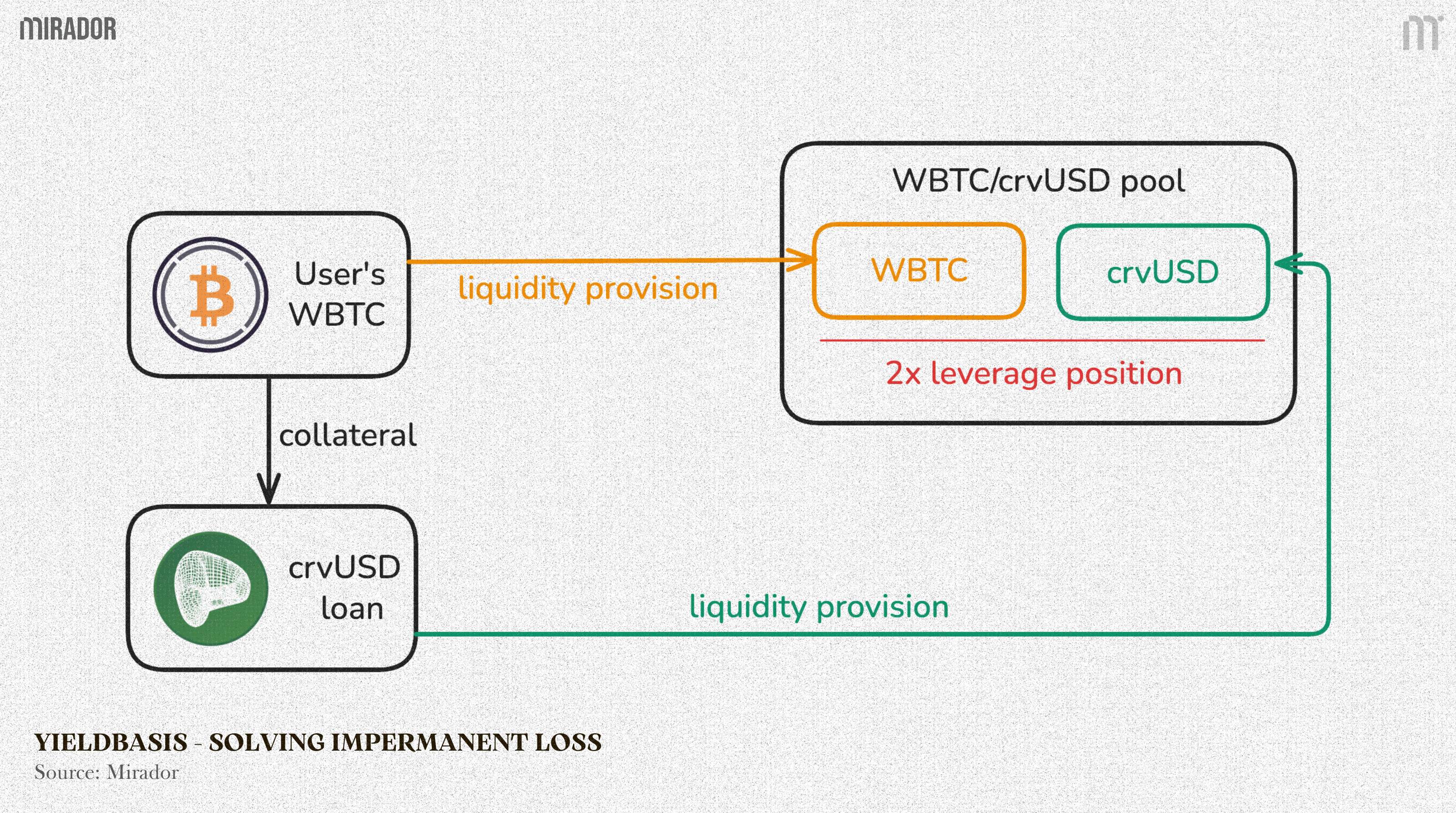
In simple terms, 2× leverage means starting with one unit of capital, borrowing one additional unit against it, and depositing the full two units into the liquidity pool. This leverage removes the square-root effect of AMMs, allowing the position to track BTC price movements more closely while continuing to earn trading fees.

This intuition is exactly what Yield Basis is designed to capture in practice. By using the initial capital as collateral to borrow stablecoins ($crvUSD) and using the original capital together with the borrowed stablecoins to provide liquidity to the pool, the protocol effectively squares the LP payoff function.

We will deeply break down Yield Basis concept to resolve impermanent loss in part II of this article.

CONCLUSION

Impermanent loss is not caused by fees, incentives, or bad market timing. It is a structural result of the constant-product AMM curve, which forces liquidity positions to grow with the square root of price changes rather than linearly.

Yield Basis addresses this problem at its root. By maintaining a constant 2× leverage through automated borrowing, repaying, and rebalancing, the protocol transforms the LP payoff from √x back into x. The result is a position that behaves like simply holding the asset, while still earning trading fees.

DISCLAIMER

In this article, we focus on breaking down impermanent loss from its mathematical foundations and explaining why it naturally arises in traditional AMM designs. Our goal is to help readers clearly understand the structural trade-offs faced by liquidity providers, and from there, build their own intuition about what it would take to eliminate impermanent loss at its root.

We do not avoid formulas or quantitative reasoning, but every step is presented in a simple and accessible way, supported by clear assumptions and intuitive comparisons, so that the underlying mechanics are easy to follow.

In Part II, we will apply this framework to Yield Basis, unpacking how its leveraged and automated rebalancing design reshapes the AMM curve. By grounding the discussion in first principles, we aim to rigorously examine whether Yield Basis can truly neutralize impermanent loss, and under what conditions this approach holds in practice.

Discussion about this post

Ready for more?