

IMPERMANENT LOSS AND HOW YIELDBASIS MAKES IT “ZERO" - PART II: “CONSTANT” 2X LEVERAGE
How Continuous Rebalancing Transforms LP Curvature into Linear Price Exposure

INTRODUCTION
“2× leverage” may sound like a simple amplification of exposure, but YieldBasis introduces something different: a continuously rebalanced leverage structure designed to neutralize the AMM’s curvature and transform the LP payoff into a linear one.
In Part I, we looked at impermanent loss from its mathematical roots. In this part II, we examine YieldBasis’ proposed solution: constant 2× leverage to make impermanent loss become zero.
KEY TAKEAWAYS
This article explores how YieldBasis constructs a constant 2× leveraged LP position, explains how it differs from simple static leverage, and then evaluates whether the strategy remains economically viable once costs are taken into account.
Section 1: Explaining the “2x leverage” introduced by YieldBasis and the difference between constant leverage and simple static leverage
Section 2: Testing Constant 2× Leverage - Accounting for Borrow and Rebalancing Costs
SECTION 1: THE BASIS BEHIND 2X LEVERAGE – THE CONSTANT LEVERAGE
In the previous article, we explained that impermanent loss in LP positions comes from the fact that price movements follow a √x pattern (where x is the token’s price change, such as WBTC).
The core to eliminate Impermanent Loss is to turn this √x behavior into a linear x movement, so that an LP position can move at the same pace as simply holding the token.
To make it happen, users’ value of a position must be changed without putting in additional capital. Of course, the most natural solution that comes to our mind is leverage.
And to address Impermanent Loss, therefore, Yield Basis’ concept is to apply leverage to effectively square the payoff function:
This is where “2× leverage” comes from.
However, thinking of it as just a 2× position is not enough, and can even miss the core idea. The section below walks through the concept in a clearer and more intuitive way.
a/ Simple static Leverage and Constant leverage
Not just 2X leverage – Must be “Constant” 2X leverage
As you think, simple 2X leverage can not eliminate Impermanent Loss
Simple static Leverage means using initial capital 𝑉_initial to borrow an additional amount D (debt), then create a LP position that is totally worth 𝑉_leverage, with:
The concept here is: You borrow once and never rebalance (debt is fixed).
At the initial time (t=0), we have:
\(V_{capital} = V_{leveraged \, LP} - D \)
When the asset value changes (t=1), debt is still fixed, we have:
\(V_{capital, \, new} = V_{leveraged \, LP, \, new} - D \)
Because debt does not change, every dollar change in LP value flows directly into your capital. This can be written as an equation of derivatives:
But since you are holding twice the LP amount relative to your initial capital, it becomes:
Integrating for total value, we have:
This means that the payoff curve is still a square-root (√P) function . It is merely shifted and scaled up in magnitude. It does not become a linear function (P).
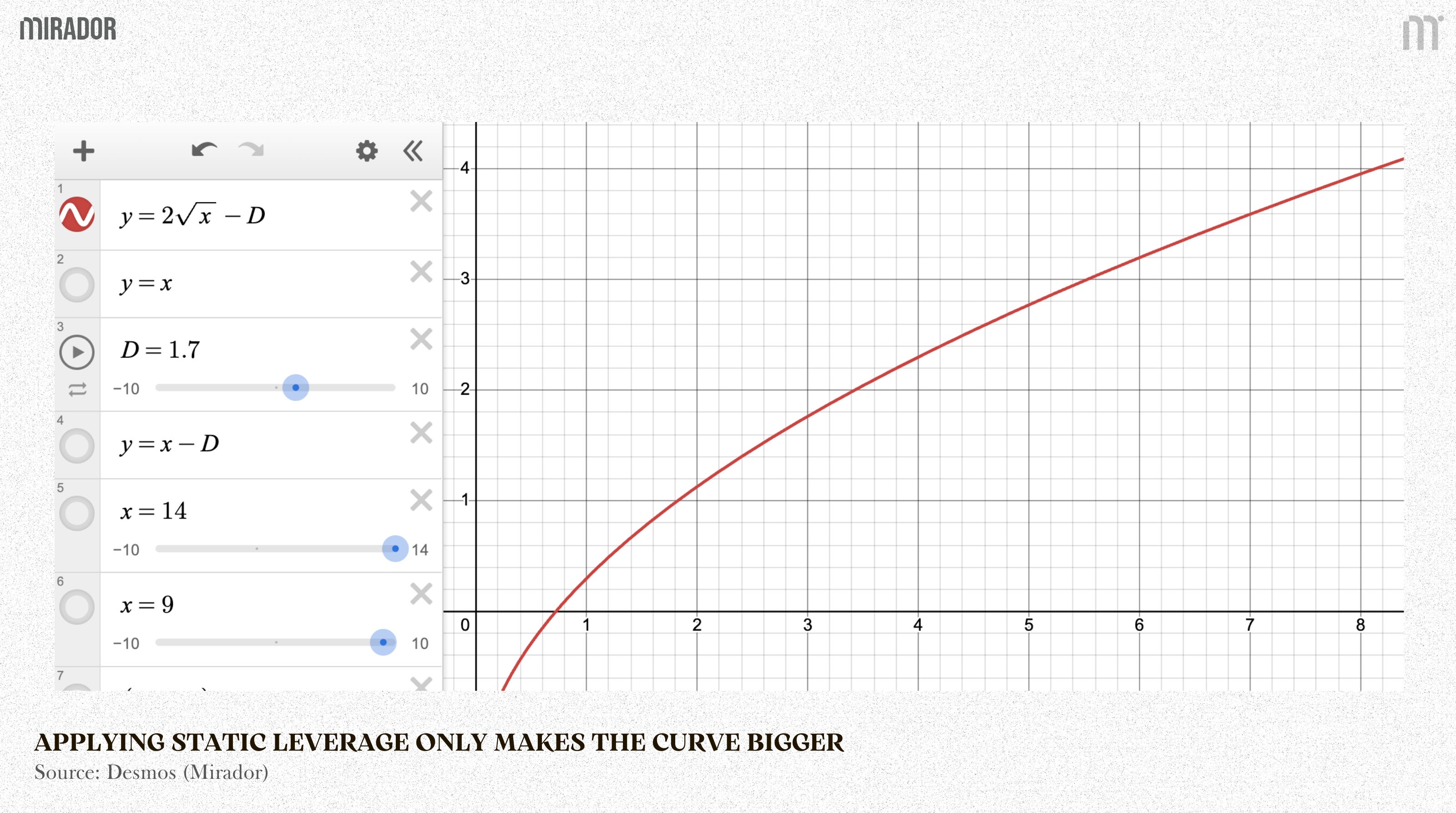
Applying static leverage (for example, 2×) only makes the curve bigger, can not change its shape
This means: The higher the price, the slower the position grows.
This can be shown mathematically with a simple derivative:
As price x increases, the derivative decreases, meaning the position becomes less responsive to further price changes.
For example: With L = 2, assume you open a position with 2× leverage:
Your initial capital: 100
Debt: 100
Total assets: 200
When the price goes up (you earn less than expected)
Suppose the asset price increases by 50%:
Total assets rise from 200 to 300
Debt remains fixed at 100
Equity becomes 200
The actual leverage is now:
Now suppose the asset price drops by 30%:
Total assets fall from 200 to 140
Debt is still 100
Equity shrinks to 40
The actual leverage jumps to:
Static 2× leverage does not maintain constant price exposure. It reduces leverage when things go well, and increases leverage when things go badly - the exact opposite of what is needed to hedge impermanent loss.
As a result, your exposure to price movements steadily decreases as the position moves in your favor. Even though the asset keeps going up, each additional price increase has a smaller impact on your equity than before.
In practice, this means leverage stops compounding returns on the upside, the 2x position increasingly behaves like an unlevered one, despite starting at 2×.
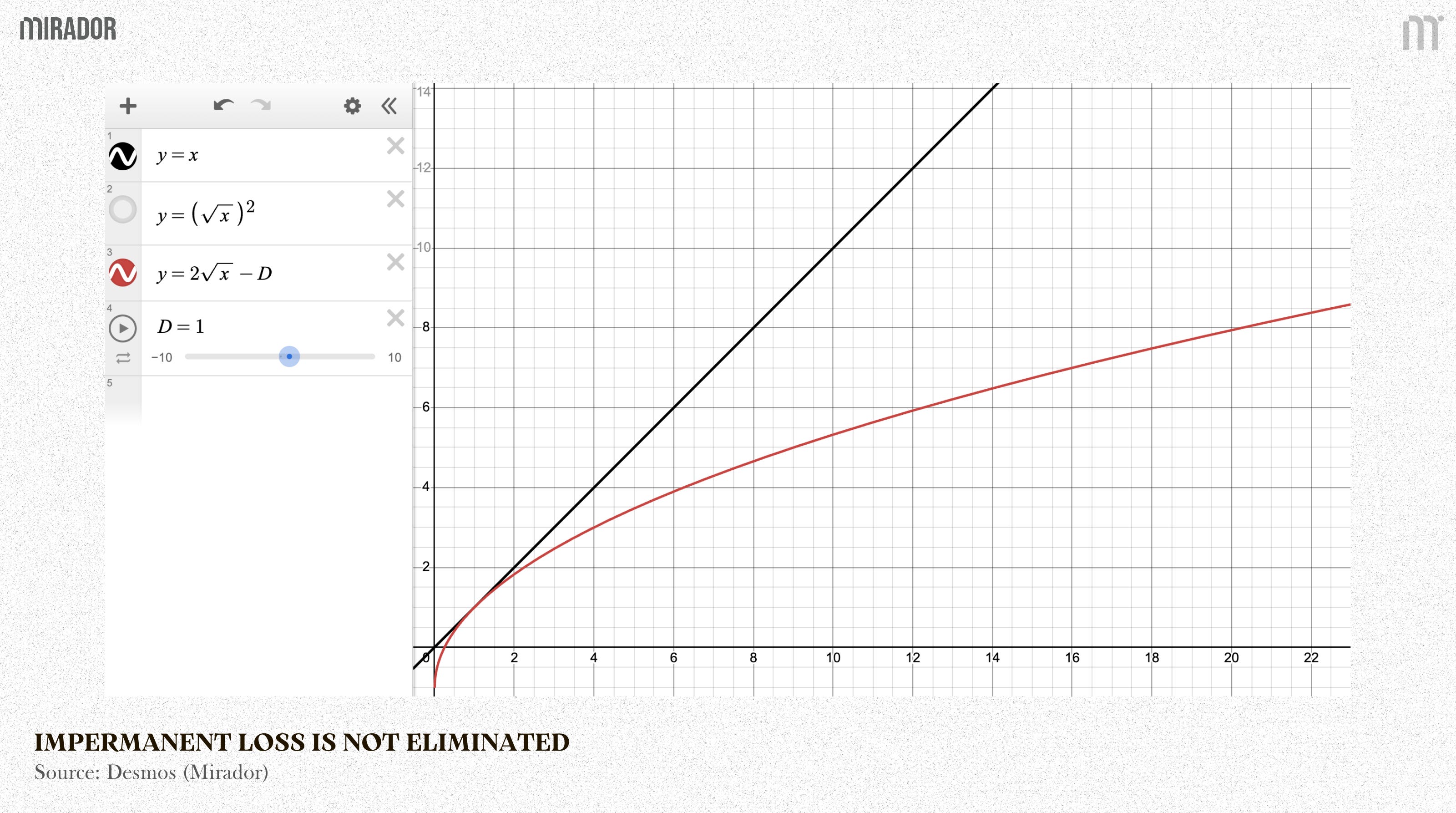
As a result, impermanent loss is not eliminated.
To turn a curve into a straight line, you cannot rely on static leverage alone. You must continuously rebalance to keep the position moving at a constant speed.
b/ YieldBasis core concept: Constant 2X leverage
Constant 2× leverage does not mean borrowing once to double your position size, instead, it means continuously maintaining a constant 2× sensitivity to price movements at every price level, not just at entry.
In other words: Static 2× leverage (which we have discussed before) just doubles your initial exposure, while constant 2× leverage keeps your price responsiveness fixed at 2×:
The position is continuously rebalanced to keep leverage level.
Borrowing amount is adjusted dynamically.
The slope of the payoff remains constant at 2.
The position moves at exactly twice the speed of the underlying price, at all price levels.
In other words, you do not commit to holding a fixed LP amount, instead, you commit to maintaining a fixed growth rate relationship.
For example: If the LP grows by 1%, your capital value must grow by 2%.
That means the position is continuously rebalanced so that your exposure always reacts at twice the speed of price, no matter where price is.
Therefore, instead of looking at absolute dollar changes, we look at relative growth:
This means the percentage growth rate of your capital is always twice the percentage growth rate of LP.
Move to logarithms:
Integrate both sides:
Using log rules:
Now substitute the LP formula of √x, now we have:
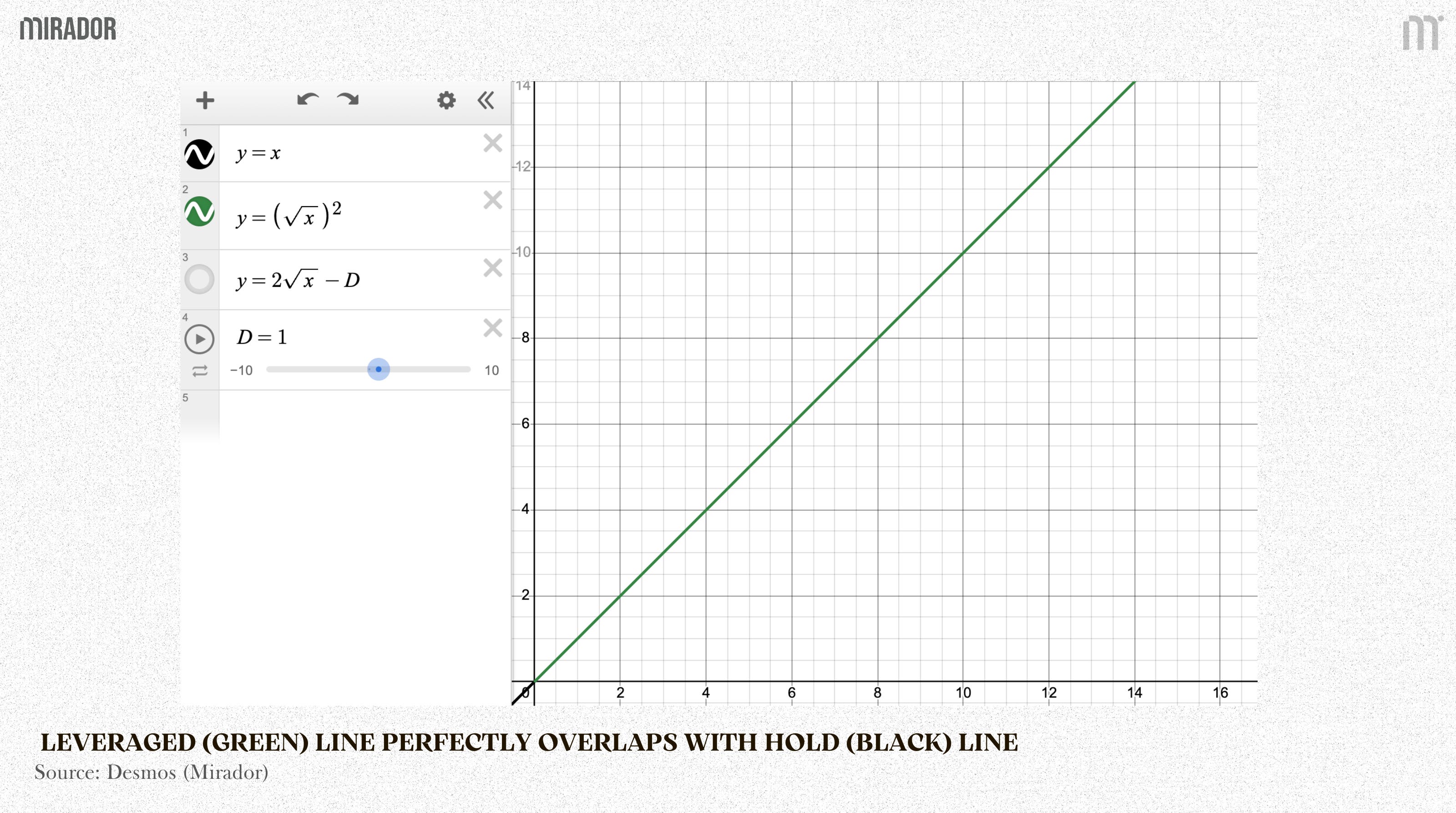
The curve now becomes a straight line; impermanent loss is eliminated:
In other words, the leveraged (green) line now perfectly overlaps with the hold (black) line. The position behaves exactly like simply holding the asset.
There is no more AMM curve effect, no divergence from holding. When the price goes up or down, the portfolio moves at the same rate as the asset itself — just like a normal spot position.
Comparison
Now, let’s put the constant 2x leverage line (green line) and static leverage line (red line) on the same graph to see the difference:
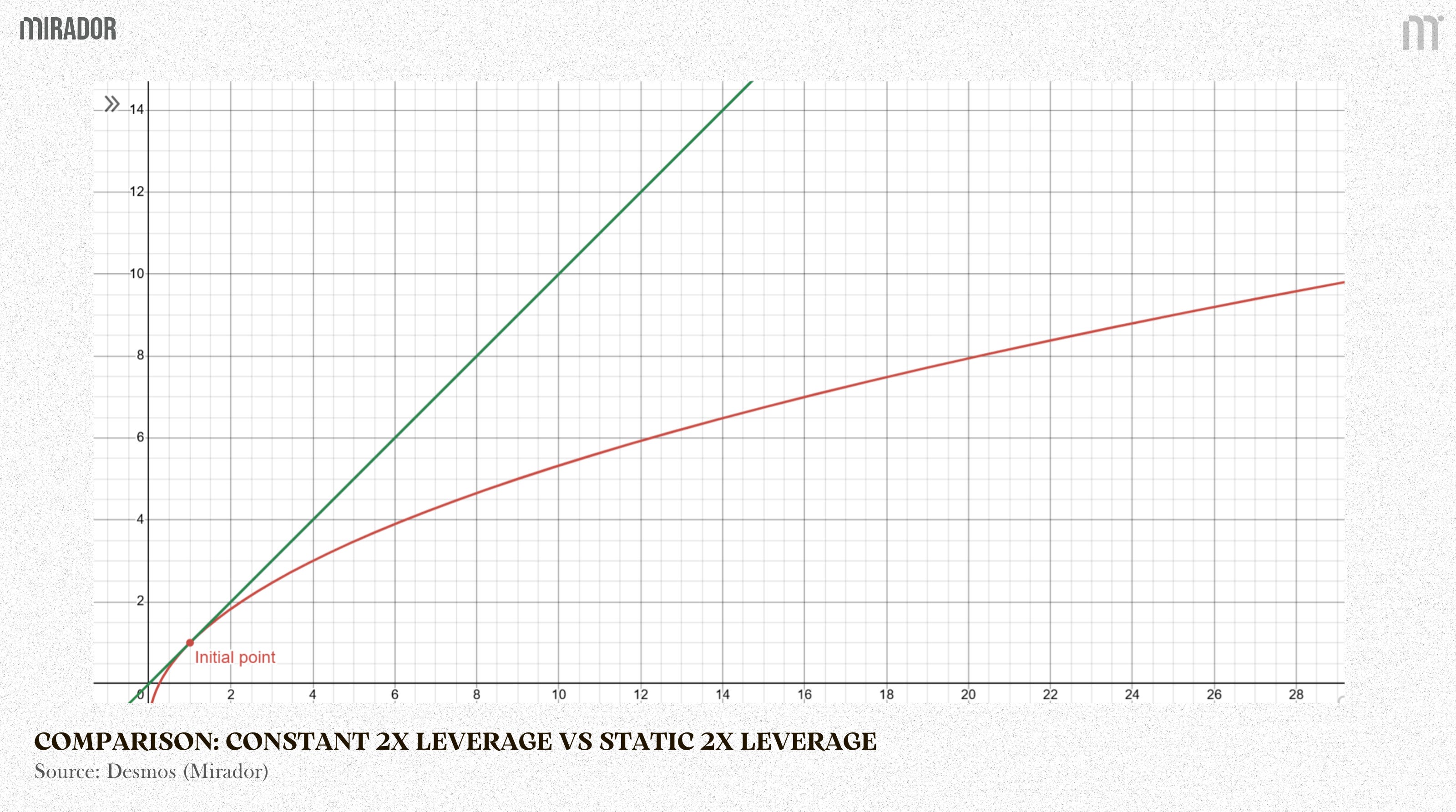
Interestingly, this shape looks very similar to the impermanent loss diagram shown in Part 1.
The Green Line (Constant 2x) is a straight line. It represents continuous rebalancing. Because the position is constantly adjusted, the LP curvature is effectively neutralized. This is the ideal outcome: the structure behaves like a simple leveraged holding, with no visible impermanent loss effect.
The Red Line (Static 2x) is curved, represents borrowing once and leaving the position unchanged. At the beginning, it closely follows the green line, but as price moves higher, it starts to bend downward and gradually falls behind.
If you compare this chart to the classic “HODL vs. LP” diagram from Part 1, the structure is almost identical.
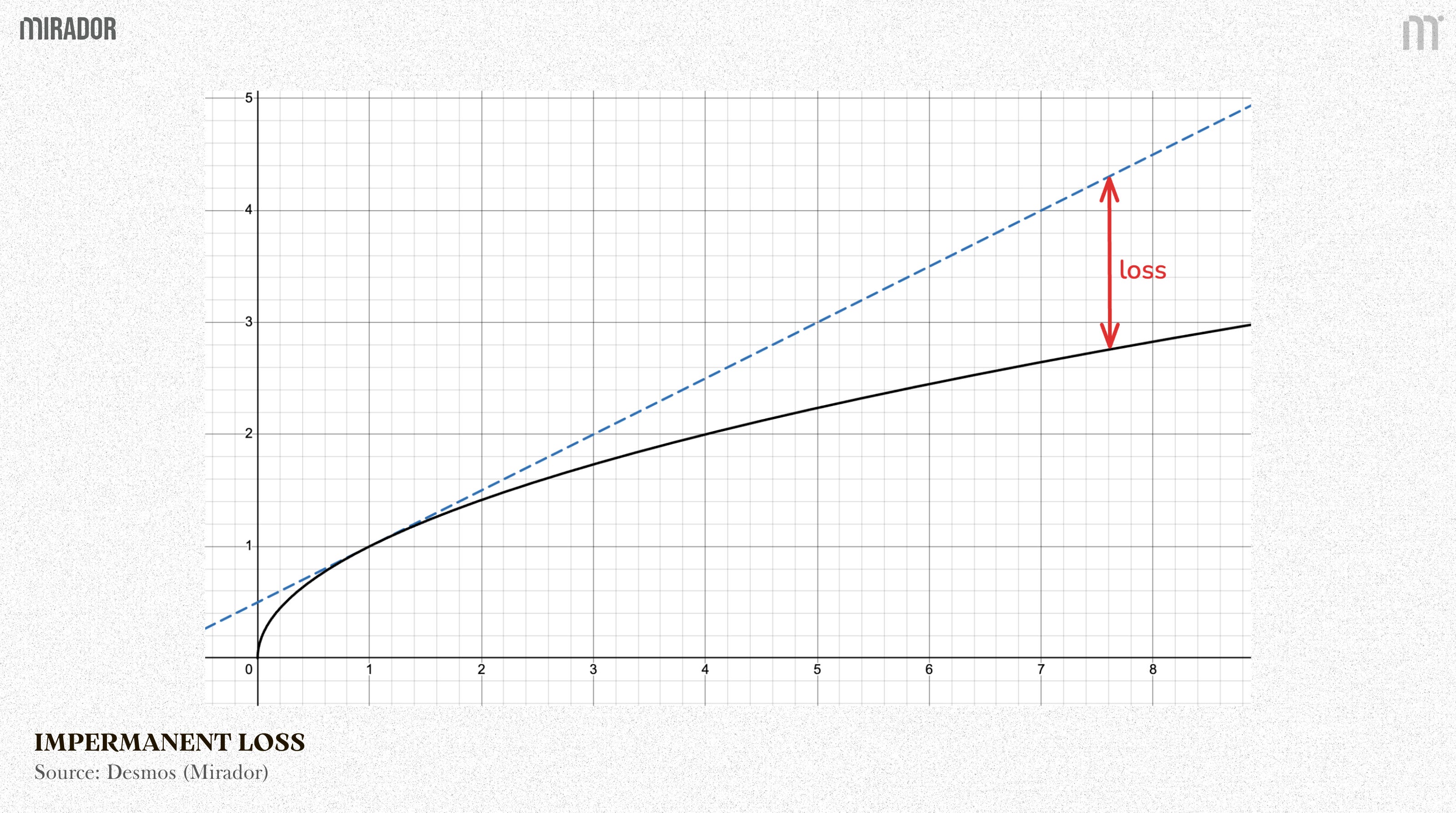
The widening gap between the green and red lines shows that static leverage does not remove impermanent loss, it is just an amplification, not a transformation.
Through continuous rebalancing, constant 2x leverage actively reshapes the exposure, effectively transforms a liquidity position into a synthetic leveraged spot holding.
However, zero impermanent loss is no free, it refers to the costs: LEVERAGING COST and CONSTANT LEVERAGING COST
SECTION 2: THE COST OF ZERO IMPERMANENT LOSS
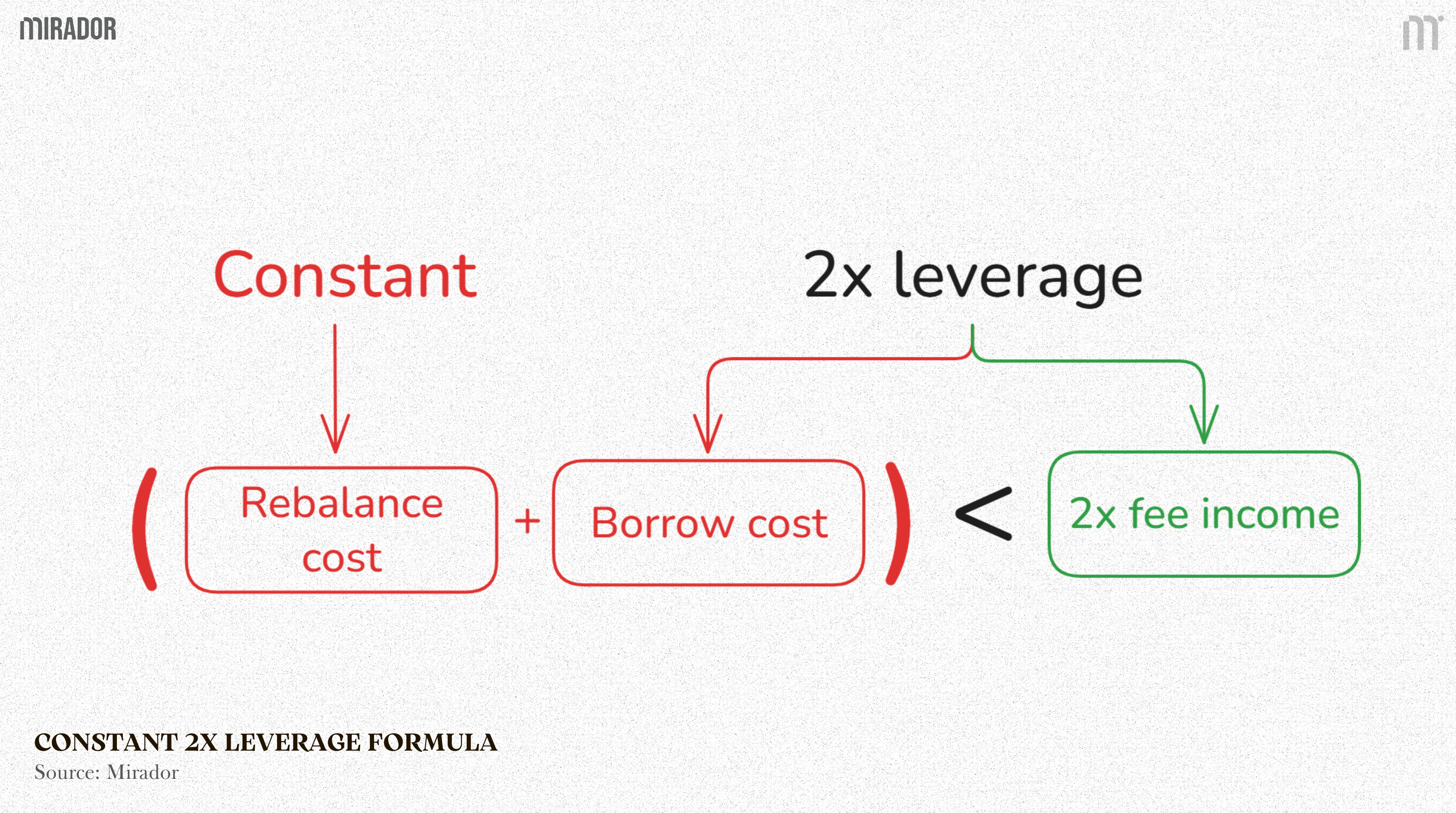
Of course, a 2x leveraged position will generate roughly twice the trading fees compared to providing liquidity with the original capital.
But consider a simple example:
Suppose you start with $100 and borrow another $100 to create a 2x LP position worth $200 (temporarily ignore overcollateralization requirements for simple understanding)
If the pool generates a 10% annual fee return, your gross fees would be $20 instead of $10, which looks attractive.
However, if the borrowing cost is 12% per year on the $100 you borrowed, that already costs you $12. On top of that, maintaining constant 2x leverage requires frequent rebalancing. Each rebalance may incur swap fees and slippage, or other additional costs...
While the fee income is amplified, the financing and maintenance costs are amplified as well. The real outcome depends on whether the extra yield is large enough to outweigh those ongoing expenses, or:

1/ Constant 2x leverage on traditional AMM: Negative PnL
To better understand how a constant 2x leverage strategy operates within YieldBasis, specifically how it interacts with a CryptoSwap pool, let’s first run a simple simulation with a traditional pool.
We model what would happen if the same constant 2x leverage logic were applied to a traditional constant-product AMM, here is Uniswap V2.
This exercise is purely illustrative. In practice, such a mechanism does not naturally exist in a standard AMM, the simulation is only meant to help us isolate and observe the mechanics of maintaining constant leverage in that environment.
The analysis breaks performance down into three simple but important drivers:
(1) Fee Income
The model looks at historical trading volume and calculates exactly how much fee income your position would have earned.
It adjusts this based on your real share of the liquidity pool over time, since your ownership percentage changes as the pool grows or shrinks.
So this isn’t theoretical yield. It’s your actual pro-rata fee income.
(2) Borrowing Cost
To maintain 2x leverage, you need to borrow capital.
The model pulls AAVE’s daily variable USDC borrowing rates and calculates the real financing cost over time. Because rates move, this captures the actual volatility of the lending market, not some fixed assumption.
This is the true cost of keeping leverage on.
(3) Rebalancing Cost
This is where most strategies quietly lose money.
To maintain 2x exposure, the position needs to rebalance whenever price moves. The model simulates those rebalancing trades day by day.
By comparing trade size against pool reserves (liquidity depth), it estimates the exact slippage and execution cost you would incur when adjusting back to target leverage.
In other words: how much value leaks out just from staying on strategy.
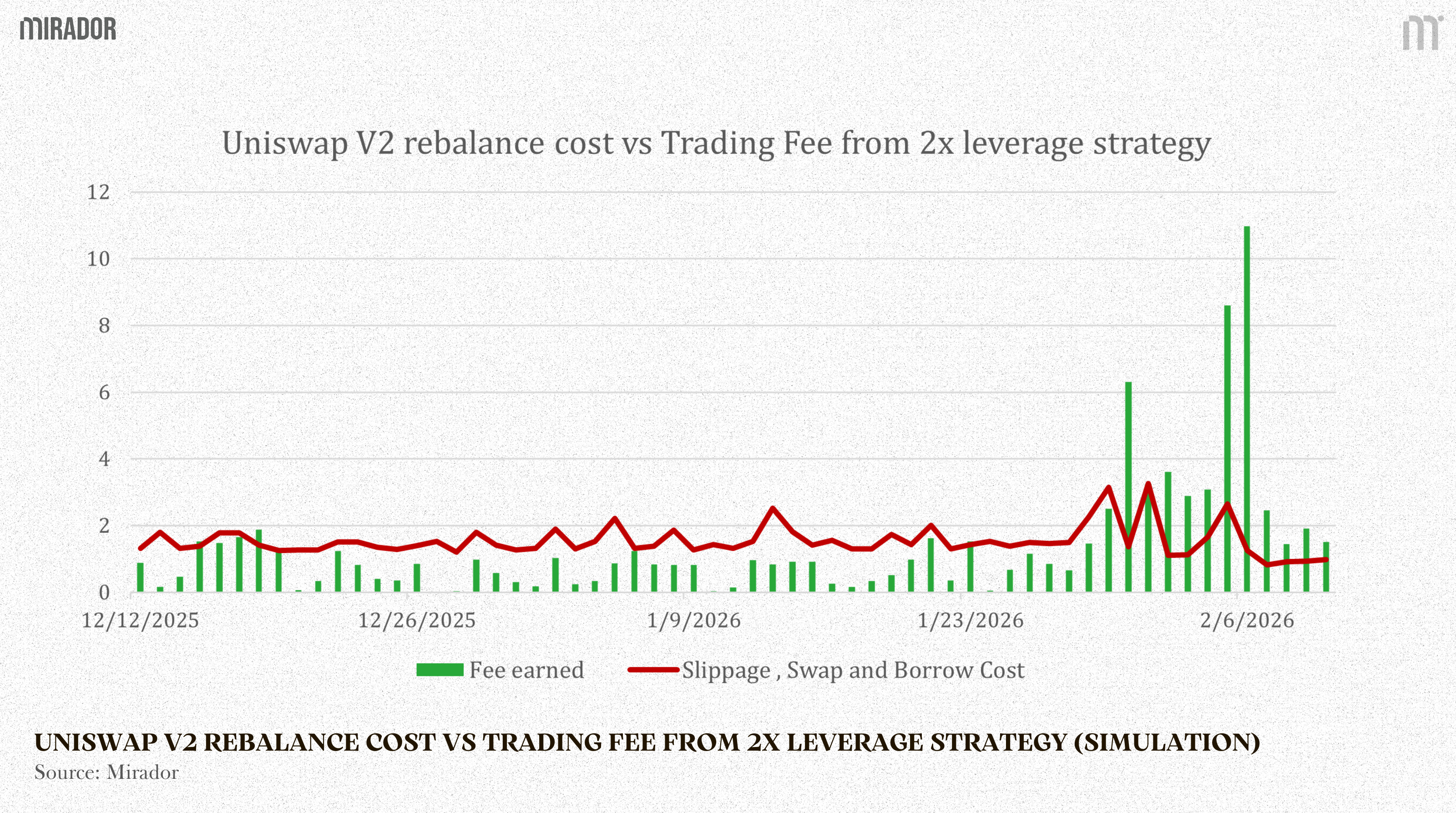
In most market conditions, the cost of borrowing stablecoins and constantly maintaining a 2x position is higher than the extra trading fees earned from using 2x leverage.
In short, the money paid for funding and rebalancing eats up the additional fee income.
The basic conclusion is that this strategy is not effective when run on a traditional AMM with high slippage. This is the primary inefficiency highlighted by the model, and the structural gap that Yield Basis uses CryptoSwap to solve.
2/ Constant 2x leverage on CryptoSwap AMM through YieldBasis
(1) Borrowing crvUSD
YieldBasis makes an LP position move 1:1 with BTC (eliminating impermanent loss) by pairing WBTC with borrowed crvUSD and maintaining a constant 2× compounding leverage.
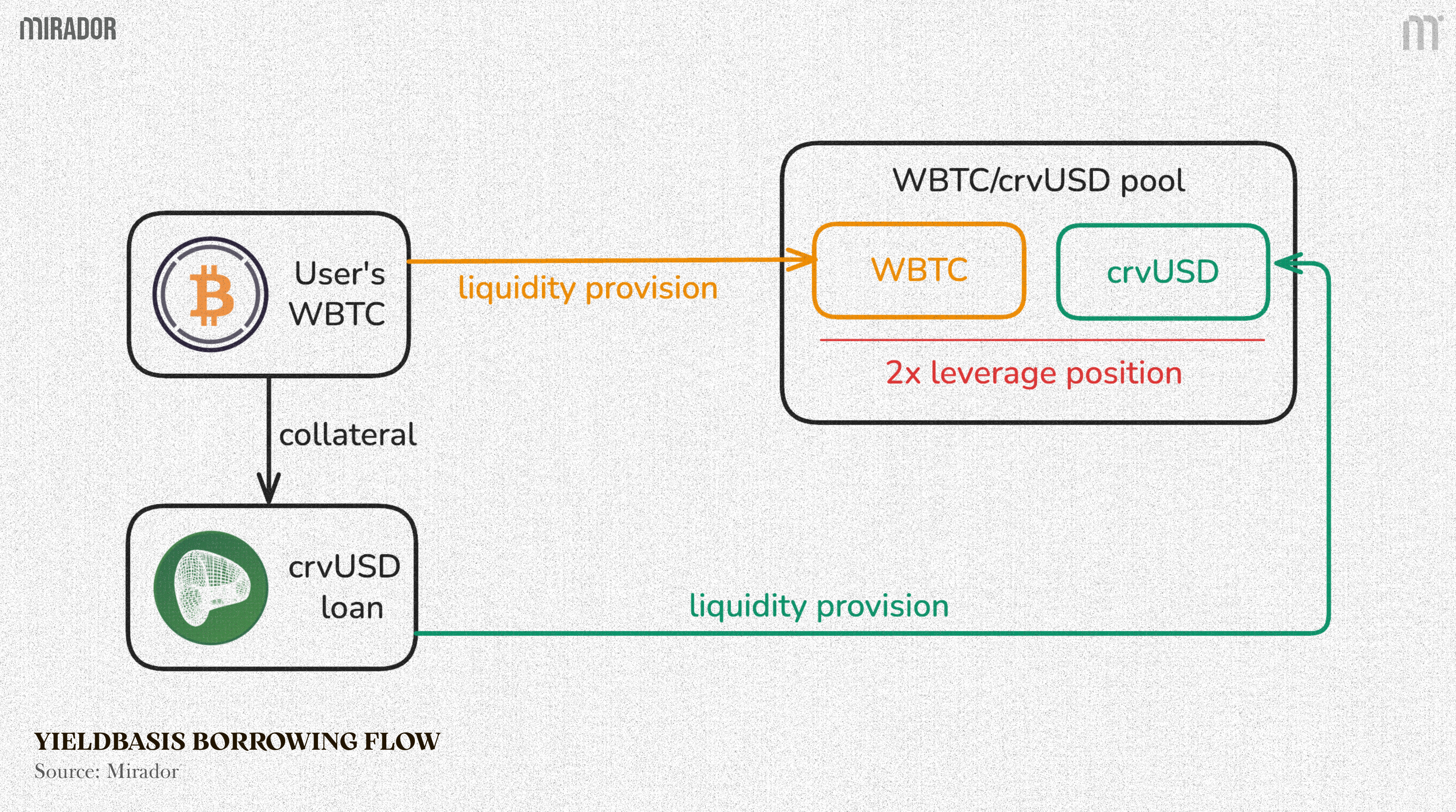
Borrow and pair: BTC is matched with an equal USD value of crvUSD, borrowed through a dedicated CDP. Both assets are then deposited into the Curve BTC/crvUSD pool.
LP as collateral: The LP token received from Curve is used as collateral for the borrowed crvUSD.
Target structure (50% debt / 50% equity): With 2× compounding leverage, debt always represents half of the total LP position value. As the LP value changes, the debt is adjusted to keep this ratio constant.
Compounding leverage mechanism: A specialized “Re-leverage AMM,” together with a virtual pool, creates incentives for arbitrageurs to step in whenever BTC price moves. Their activity automatically pushes the position back to the 2× leverage target
(We will deeply diving into it in part 3 of this article)
As a result, the LP exposure is continuously reshaped so that it behaves like holding BTC spot with 2× leverage, but without the typical impermanent loss curve.
(2) Rebalancing to keep 2x leverage
Rebalancing basis: Borrow and Repay
In practice, the position is continuously adjusted by either repaying or borrowing additional crvUSD. When the BTC price moves, the value of the LP position changes, which causes the leverage ratio to drift away from its target. To correct this, the system:
Borrows more crvUSD when leverage falls below the target, using the borrowed stablecoin to increase exposure.
Repays crvUSD debt when leverage rises above the target, reducing risk and restoring balance.
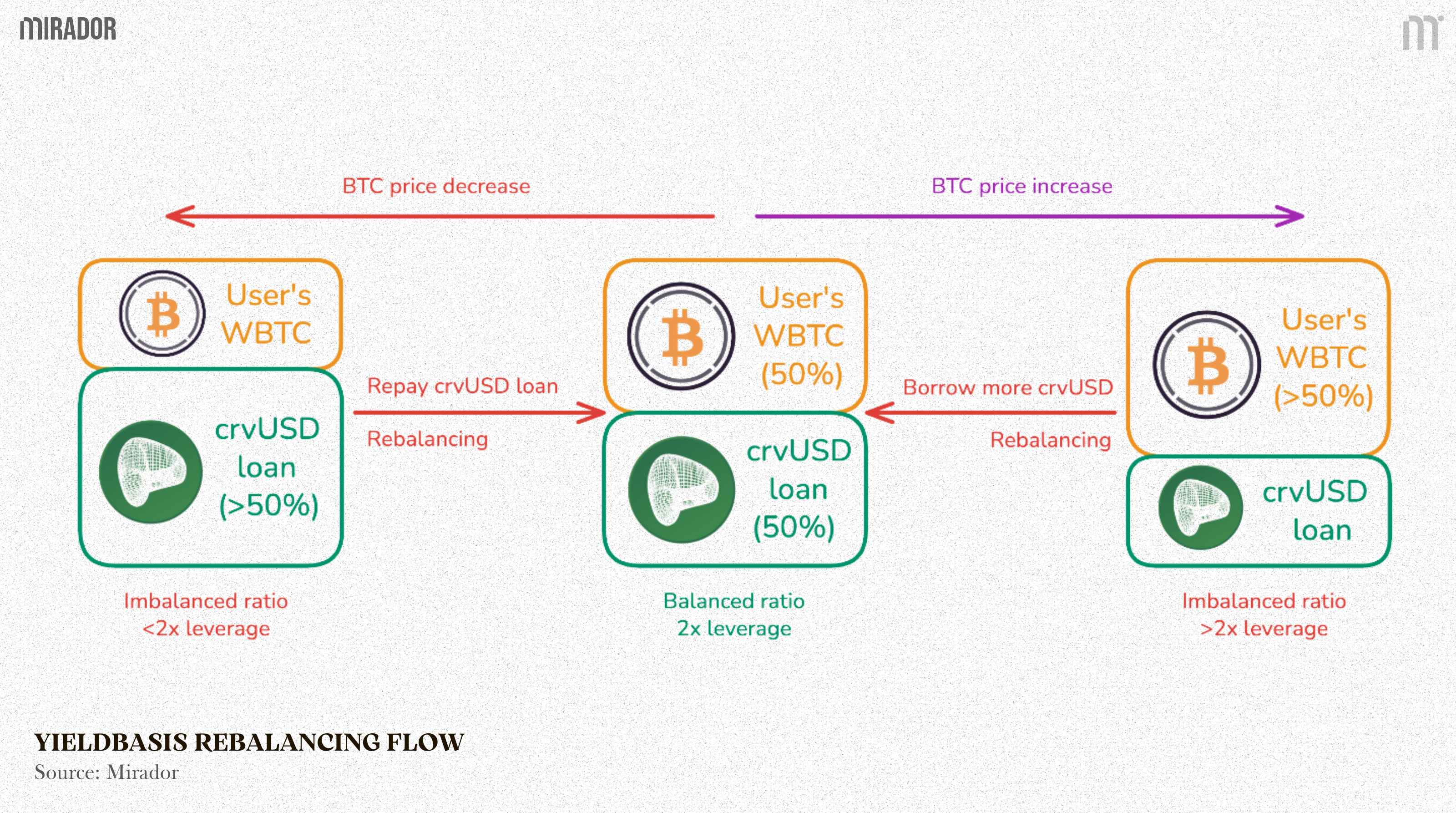
This process ensures that the position stays close to its intended leverage, most importantly, the 2× target that neutralizes impermanent loss and preserves linear price exposure. The rebalancing mechanism is designed to be mechanical and capital-efficient, relying solely on crvUSD flows without requiring users to manually intervene.
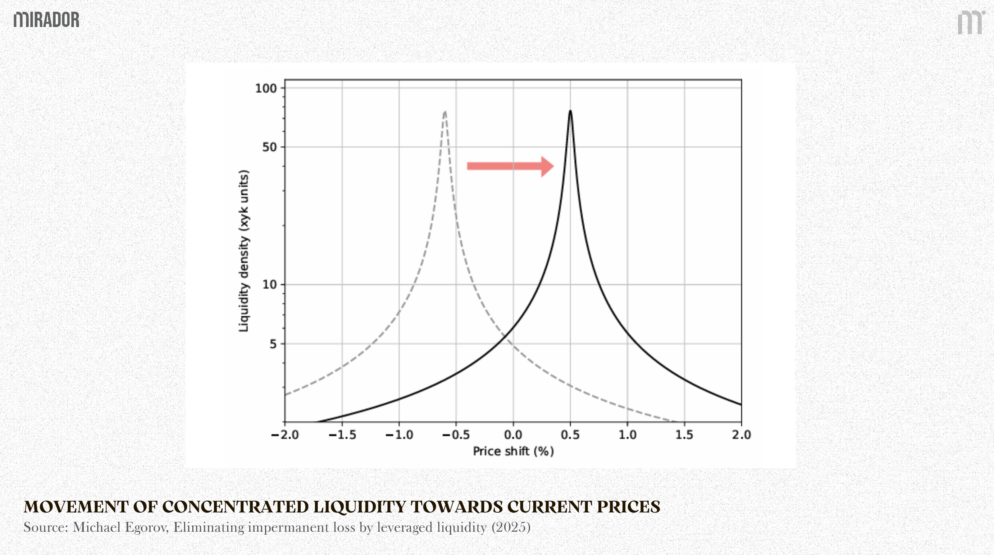
(3) Rebalancing to concentrate liquidity (CryptoSwap pool)
Curve’s CryptoSwap uses concentrated liquidity, meaning capital is focused around a specific price range rather than spread evenly across all prices.
This design improves capital efficiency, but it introduces a challenge: When the market price moves away from the center of concentration, liquidity becomes less effective.
To restore efficiency, the protocol must shift the peak of the liquidity curve toward the new market price.
However, moving the curve is not free.
Re-centering liquidity requires trades against the pool, and those trades create a real economic loss. Therefore, the system needs a budget to pay for this adjustment.
Previously, this adjustment budget came from trading fees generated by the AMM, but it only works when trading volume is strong.
In YieldBasis, it is improved by using crvUSD borrow fee as part of liquidity adjustment budget: Rather than treating borrow interest as isolated revenue, the system redirects part of this continuous cash flow into the liquidity adjustment budget.
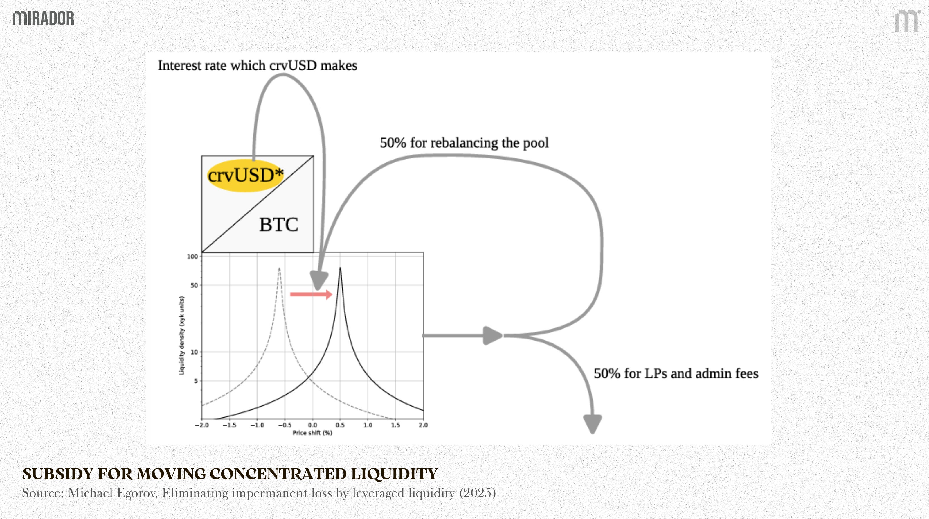
The protocol splits borrow fee paid by user:
50% goes to LPs/admin
50% is allocated as a subsidy for moving concentrated liquidity
This subsidy directly finances the cost of shifting the liquidity curve toward the new market price.
(4) Simulation with total cost
In this simulation, we found the answer for question “If I invest $1 million into the WBTC/crvUSD (YB) pair using 2x leverage, how much real profit would I have made per day over the past 60 days after deducting borrowing interest and all price-related losses?”
Important note: The Curve and Uniswap V2 simulations use different pairs and position sizes.
Curve test: WBTC/crvUSD with $1,000,000 capital.
Uniswap V2 test: WBTC/USDC with $10,000 capital.
This adjustment was necessary because Uniswap V2 does not have enough reliable historical data for WBTC/crvUSD, and its liquidity is much lower.
The smaller $10,000 position ensures the backtest reflects realistic market depth and avoids distortions from running large trades in a shallow pool.
This analysis runs a full 60-day historical backtest to measure the actual net profitability of a 2x leveraged liquidity strategy on WBTC/crvUSD.
From the implications discussed in part (c), we construct a simplified simulation model to evaluate the sustainability of constant 2× leverage.
The model combines on-chain data to break performance into three core components:
(1) Trading Fee Revenue (Gross Yield)
It aggregates daily trading volume and TVL to compute the Capital Turnover Ratio, which estimates how much gross yield is generated from trading fees.
(2) Rebalancing & Slippage Cost (Execution Drag)
To measure execution efficiency, the model compares actual trade prices with oracle reference prices (Chainlink/internal) on a minute-by-minute basis.
This captures the “hidden cost” of slippage — in other words, how much value is lost when the strategy rebalances during price divergence.
(3) Borrowing Cost (Cost of Capital)
It tracks the variable on-chain borrowing rates of the collateral assets to calculate the exact interest expense required to maintain 2x leverage.
For clarity, we do not treat the liquidity-movement subsidy as a separate expense. It is already internalized within the borrow cost.
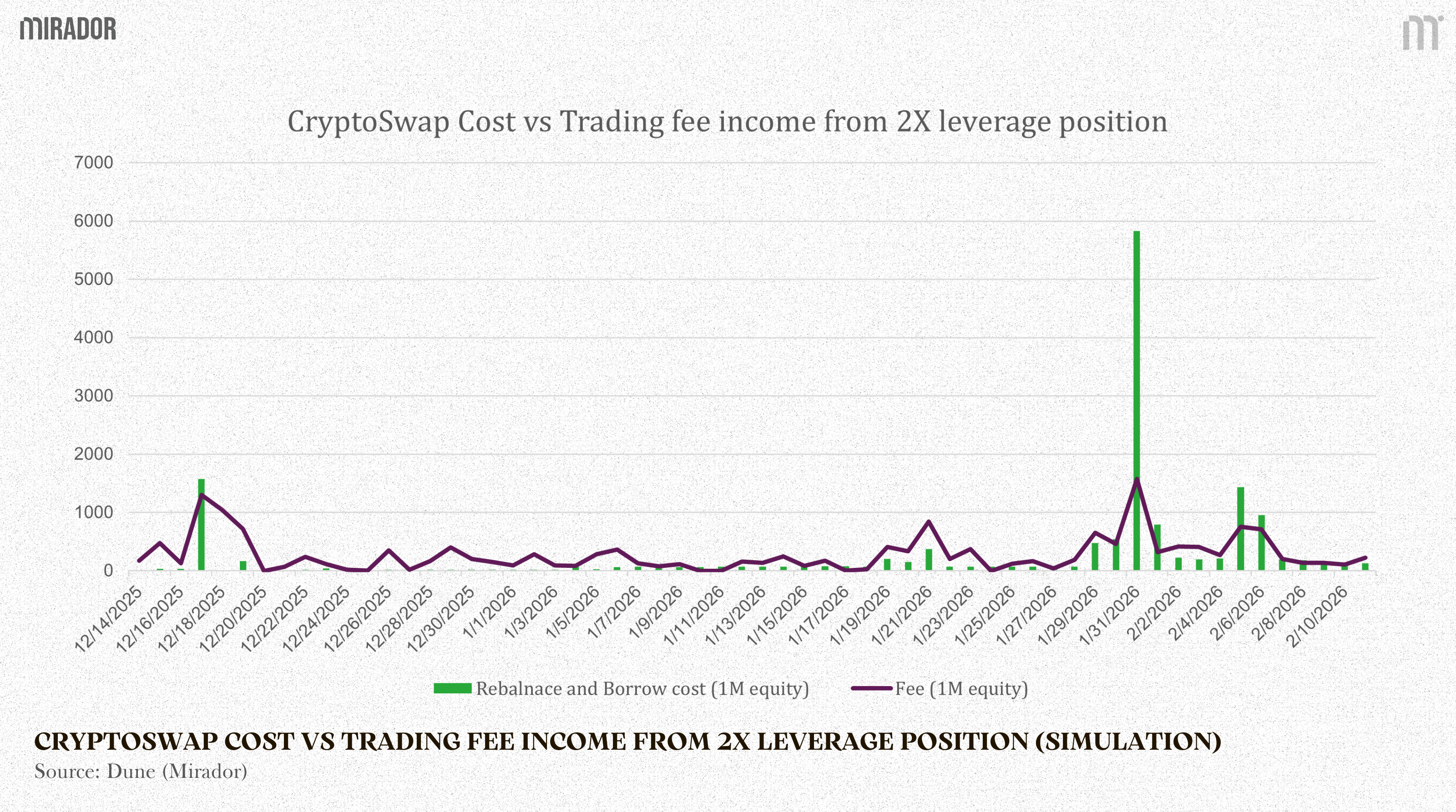
In this Yield Basis test model, fee income is higher than costs in most market conditions.
For the majority of days, trading fees from the 2x position exceed the combined rebalancing and borrowing costs. This means the strategy is generally net positive under normal volatility and volume conditions.
However, there are specific stress periods where costs spike sharply, typically during sudden market moves. In those moments, rebalancing becomes expensive and can temporarily exceed fee income.
CONCLUSION
YieldBasis’ constant 2× leverage demonstrates an important insight: Impermanent loss is not unavoidable, it is structural, and therefore, it can be engineered around.
By continuously maintaining a fixed leverage ratio, the system effectively squares the AMM payoff curve, transforming √x into x. The LP position no longer drifts away from holding, it becomes straight.
In Part III, we will dive deeper into the mechanics of how this transformation is implemented at the protocol level.
Disclaimer:
In this article, we approach YieldBasis’ constant 2× leverage from first principles. Rather than taking “zero impermanent loss” at face value, we examine the mathematical logic behind it and test whether the mechanism truly reshapes the AMM curve as claimed.
Our goal is not to advocate or criticize, but to understand the structure: what works in theory, what depends on assumptions, and where real-world costs enter the picture.
In Part III, we will move beyond equations and explore how this transformation is implemented at the protocol level, and whether the design can remain sustainable in practice.