

PENDLE AMM - THE HIDDEN ENGINE OF YIELD TRADING PART I: POTENTIAL AMMs FOR TRADING FIXED YIELD
Understanding the AMM designs that previously enable on-chain fixed yield trading before Pendle V2 AMM

INTRODUCTION
Pendle Finance is currently the largest yield trading protocol in the decentralized finance space. For trading operations to run smoothly, flexibly and securely, the Automated Market Maker (AMM) model is needed to secure this.
This first part of the series does not focus on Pendle V2’s implementation itself immediately. Instead, it builds the conceptual foundation by examining the AMM models that historically made on-chain fixed yield trading possible by exploring how different invariant designs attempt to price Principal Tokens (PTs).
KEY TAKEAWAYS
In Part 1 of this series, we introduce and explain some potential AMMs for trading PT token with fixed yield, including:
Section 1: Constant Geometric
Section 2: YieldSpace’s constant power sum
Section 3: Notional’s AMM model (basis of Pendle V2 AMM)
Section 4: Comparison of Fixed-Yield AMM Models
PRIMARY PROBLEM: HOW PT PRICE CAN BE TRADED THROUGH AUTOMATED MARKET MAKERS (AMM)
Essentially, trading PT means selling PT to receive its underlying asset or buying PT using its underlying asset.
In the Pendle context, we understand the transaction of trading a PT token will be handled by a specific pool of SY and PT, where users could trade one for the other, or provide liquidity to it.
For example, transactions of buying or selling PT-USDe will be handled in the SY-sUSDe/PT-sUSDe pool.
This means that even if you sell PT token for another token that’s not its underlying token, or vice versa, a swap transaction will firstly happen.
For example: Say I want to buy PT-sUSDe but using WETH
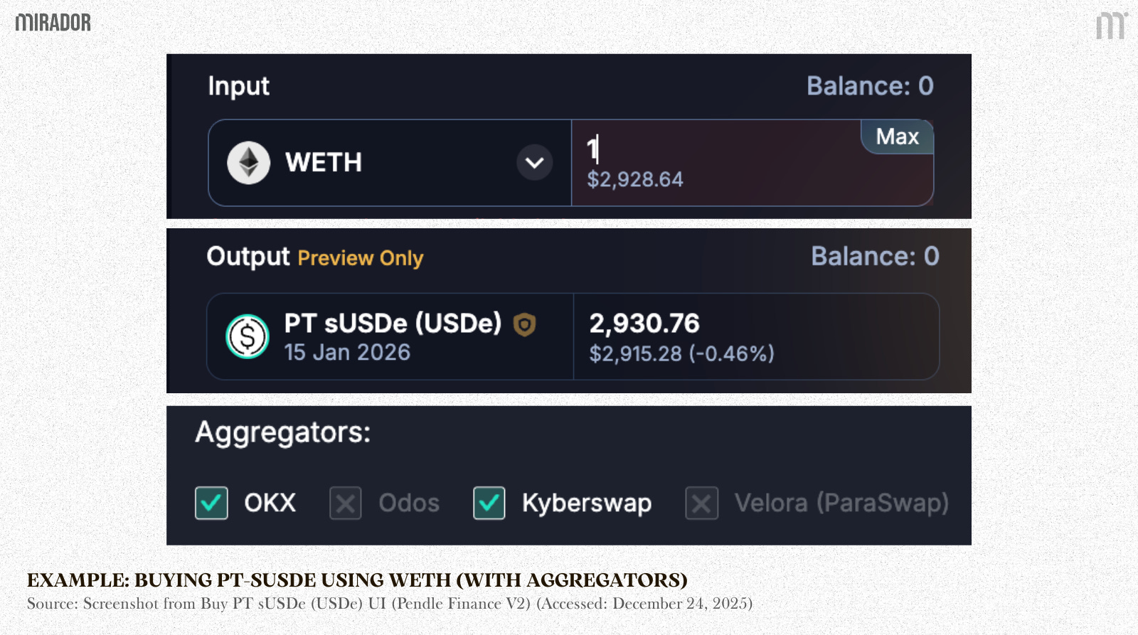
The in-amount of WETH is routed to other DEX (for example, Uniswap V3) by DEX aggregators, the swap process ends up with the same amount of sUSDe.
Finally, Pendle converts these sUSDe to SY-sUSDe and AMM will calculate the out-amount of PT-USDe for my transaction.
Therefore, the relationship between PT and its underlying asset is similar to 2 tokens X,Y in a normal DEX liquidity pool and follows a very simple AMM logic: Buy more X will make it become more expensive, which is called slippage.
From now on, we have the notation as:
X: the number of asset in principal (nasset) (in Pendle, X is nSY), with price called pricea
Y: the number of PT token (nPT-asset), with price called pricep
With:
pricea is the price of the asset in terms of principal token
pricep is the price of principal token in terms of asset
For example: AMM in the SY-sUSDe/PT-sUSDe pool will have SY-sUSDe as token X and PT-sUSDe as token Y, if:
pricea(t)=1.05, which means you need 1.05 PT-sUSDe to buy 1 sUSDe at time t
pricep(t)=0.95, which means you need 0.95 sUSDe to buy 1 PT-sUSDe at time t
(t (year) is the remaining time until maturity)
It is simple to see that at time t:
Traditional AMMs like Uniswap or Curve are designed to keep token prices balanced around a constant invariant. That works well for regular tokens but Principal Tokens (PTs) behave very differently:
PT is redeemable for a fixed amount of assets after expiry, 1 PT allows users to get back 1 asset worth after the expiry.
PT price before maturity is the discounted price of underlying asset
For example:
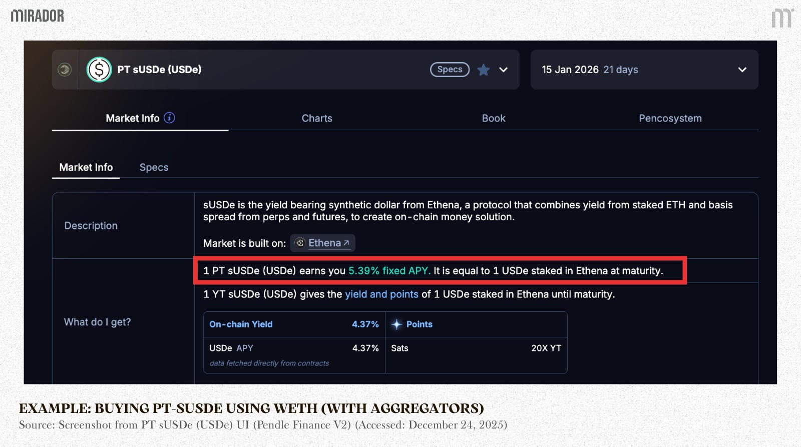
1 PT-sUSDe-15th Jan 2026 will be redeemable for the principal of 1 sUSDe after 15th January 2026.
At the time of writing, its price is equal to 94.61% of the price of sUSDe, meaning buying PT-sUSDe now will earn me 5.39% fixed yield.
Or in other words, it costs me 0,9461 sUSDe to get 1 sUSDe at maturity.
This means that the price ratio of PT to its underlying asset (ratio of Y to X; or in Pendle, PT to SY) is changing over time (because t is always decreasing and will be 0 at maturity), and reaches (1:1) at the maturity date.
While the famous AMM invariants (Uniswap with constant product invariant, or Curve with StableSwap,...) are designed to keep the price ratio of X to Y stays remain, PT needs another AMM math to effectively gradually “pull” its price to SY price until maturity.
The logic of PT Trading:
Because of slippage, buying PT will increase pricep(t) and decrease pricea(t), which means decreasing the implied interest rate (decreasing fixed yield).
Conversely, selling PT will decrease pricep(t) and increase pricea(t), which means increasing the implied interest rate (increasing fixed yield).
SECTION 1: CONSTANT GEOMETRIC
This model is used in Pendle V1 AMM, which uses a weighted product formula to manage its liquidity and determine asset prices.
This model is defined by the core formula (the invariant):
With:
X and Y are the amounts of the two assets in the pool (PT and underlying asset)
Wx and Wy are the “weights” or “importance” of each asset (they must add up to 1, as shown above).
k is the “constant” value, this value must remain the same after every trade.
Essentially, Uniswap V1 and V2 AMM (x*y=k) is also a special case of this formula where the weights are equal (Wx=0.5 and Wy=0.5).
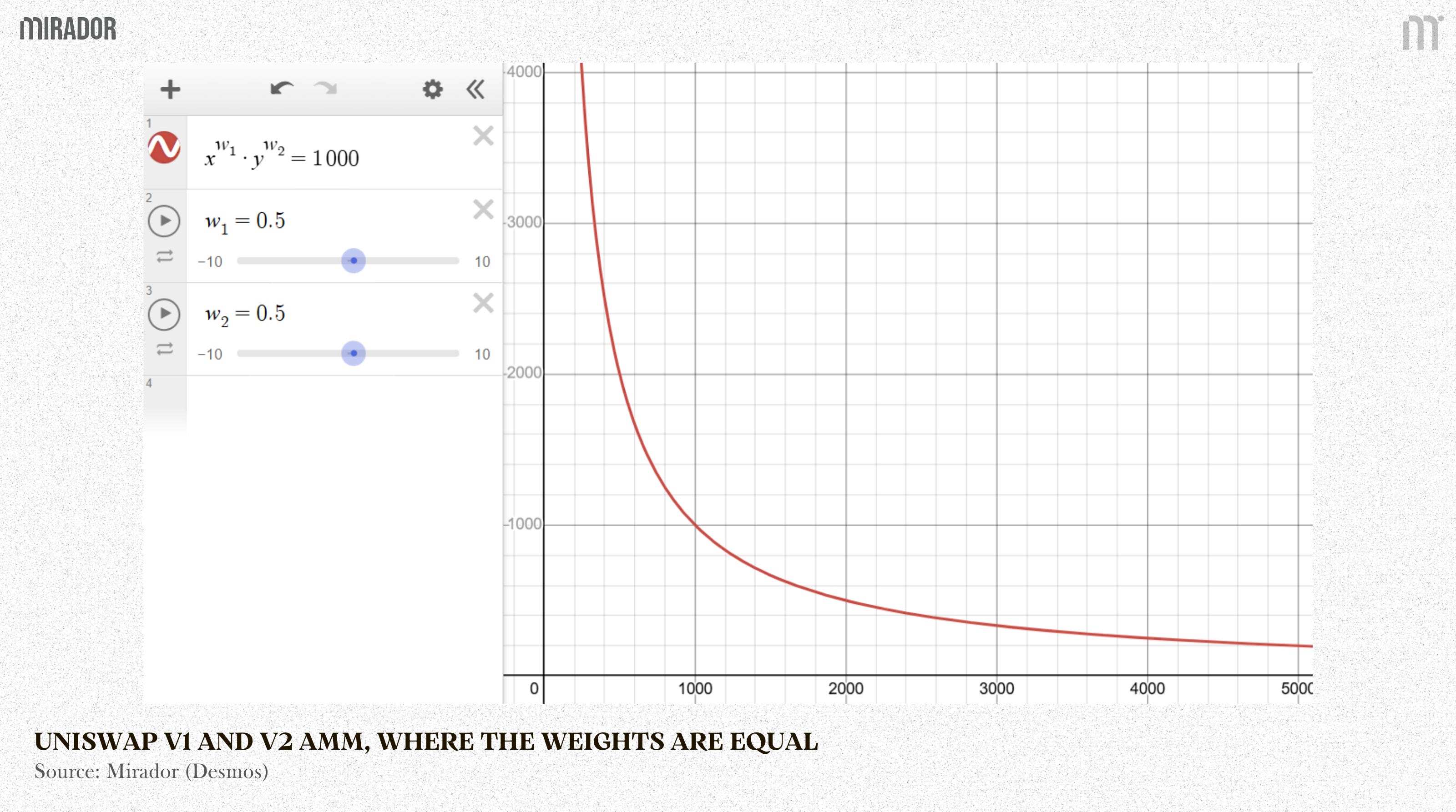
By giving the assets different weights, this model allows for more flexible and customized pricing curves.
In PT AMM, the most important thing is to pull the pricep(t) and pricea(t) to 1 (which means 1 PT = 1 underlying asset) when it reaches the maturity date, regardless how many X and Y are there in the pool.
Therefore, the weight parameters are added and adjustable:
As the maturity date comes closer overtime, Wx gets closer to 0 and Wy gets closer to 1. This makes the price curve gradually become flatter and nearly a straight line at maturity, making the price ratio turn into (1:1).
And because assets’ weights are changing continuously, even if there’s no transaction making x and y vary, PT’s pricep(t) still increases over time and ends up at 1.
SECTION 2: YIELDSPACE’S CONSTANT POWER SUM
YieldSpace’s “constant power sum” is a smart AMM formula designed to automatically change an asset’s price over time. Its main purpose is still to trade a PT against its underlying asset, making sure the PT’s price automatically rises to 1 at maturity.
Its core formula is:
With:
X and Y are the amounts of the two assets in the pool (PT and underlying asset)
k is the “constant” value, this value must remain the same after every trade.
t is the time left until maturity (it is standardized to go from 1 down to 0).
This formula is smart because it automatically changes the shape of the pricing curve as t changes.
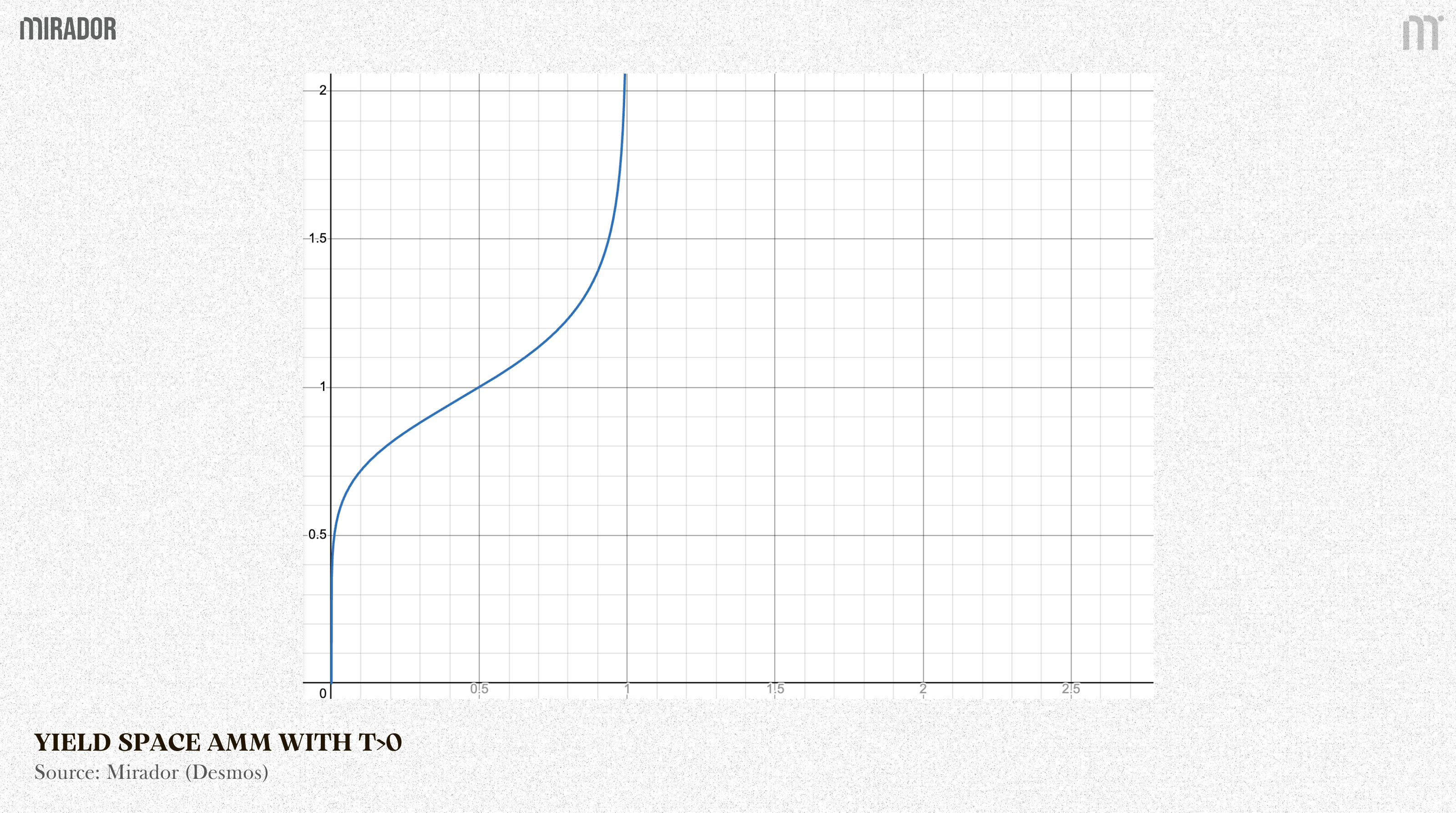
Scenario 1: Far from maturity (t>0)
We have:
Asset price in principal, pricea(t) shows how the PT amount changes when the base asset changes. Therefore, to calculate it, we take the derivative of y with respect to x, which is dy/dx.
Buying PT means a trader adds more of the underlying asset to the pool, so the pool must release some of the other token (PT) to keep the invariant constant, which means y < 0 and x > 0.
Conversely, selling PT means dy > 0 and dx < 0
Therefore, dydx is always a negative number
So that:
Taking derivatives:
After mathematical transformation, we have:
When t gradually decreases from 1 down to 0, (yt)t also reduces to (yt)0=1, meaning the pricea(t) decreases to 1, or pricep(t) increases to 1
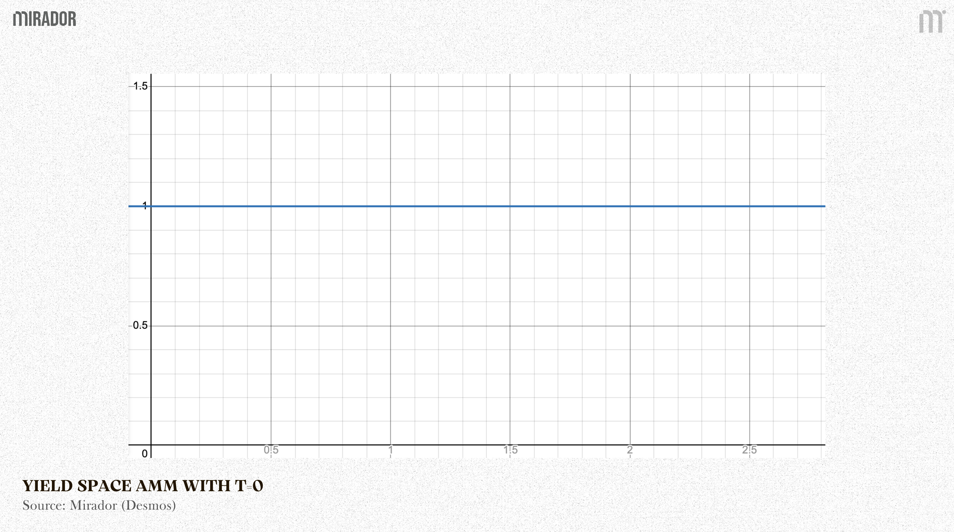
Scenario 2: At Maturity (t=0).
The formula becomes constant sum invariant, as known as the complete zero slippage invariant:
X+Y=k
It’s a straight line, meaning 1 X always equals 1 Y, 1 PT = 1 asset or pricep(t) = pricea(t).
SECTION 3: NOTIONAL AMM
Notional AMM is the basis of Pendle V2 Yield Trading AMM.
Instead of determining that the total amount of PT and underlying assets must satisfy a certain invariant formula, Notional directly defines the price of the base asset in PT terms follows a specific formula:
With:
rateAnchor (t) is the price (expressed as an interest rate) that the pool thinks is the correct market price. It acts like a moving “anchor” that the price is tied to and it’s adjusted before every trade to follow the real market.
As the maturity date gets closer, the rateAnchor automatically moves toward a 0% interest rate (meaning pricea(t) = 1).
rateScalar (t) controls how much liquidity is concentrated at the rateAnchor price.
It’s calculated as:
As time t gets smaller (near maturity), rateScalar becomes huge.
ln(p(t)1-p(t)) measures how unbalanced the pool is. When you trade, you change the pool’s balance, and this term creates the slippage.
p(t) is the proportion of PT in the pool at time t, therefore, p(t)1-p(t) is the ratio of PT and its underlying asset
From that price formula, they then derive how the pool’s x and y reserves change during a trade.
To make it easier to understand, let’s see how the parts work together:
Scenario 1: Far from maturity (t is big)
Because so rateScalar is small with big t.
Slippage is equal to ln(p(t)1-p(t)) dividing by a small rateScalar, making the slippage HIGH

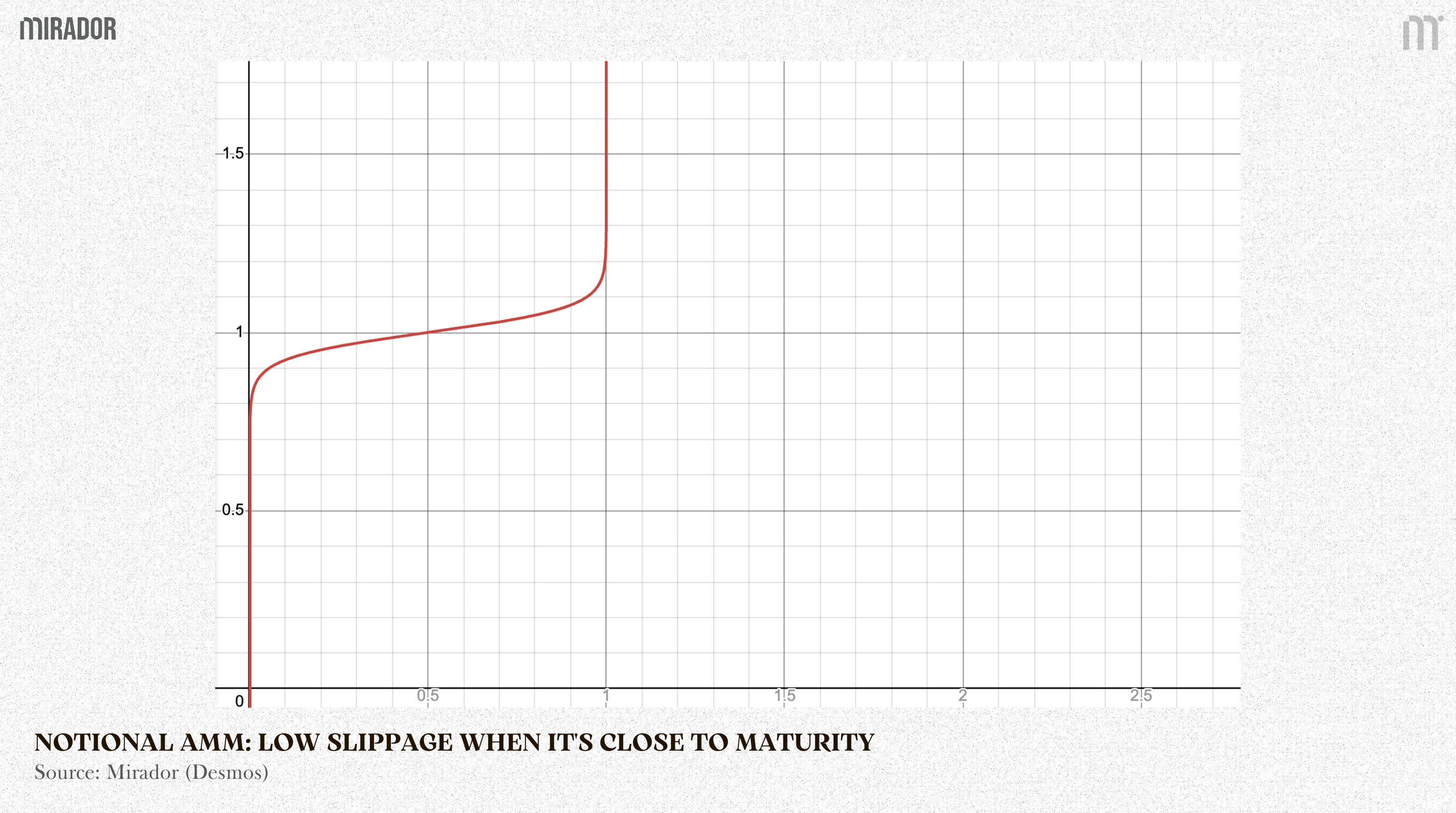
Scenario 2: Near maturity (t is small), so rateScalar is huge.
Slippage is equal to ln(p(t)1-p(t)) dividing by a huge rateScalar makes the slippage TINY (slippage almost zero on maturity).
DECTION 4: COMPARING: NOTIONAL AMM IS THE MOST CAPITAL EFFICIENCY
As we have discussed, all of three models are able to “pull” PT price to asset price on maturity date. Therefore, to determine which is the most effective model for PT trading, let’s compare the capital efficiency of these three AMMs at the same point of trading.
To compare the effectiveness of each model for PT trading, we can see how the pricea(t) (price of asset/principal token) moves when users buy or sell principal tokens.
In graphic illustration, we called it “a”.
In Constant Geometric model, we have:
\(price_a = \frac{w_x}{w_y} \times \frac{y}{x} \quad \frac{p}{1-p} = \frac{y}{x}\)
So that:
In YieldSpace’s model, we have:
In Notional’s model, we have
\(price_a(t) = \frac{ln \left( \frac{p(t)}{1-p(t)} \right)}{rateScalar(t)} + rateAnchor(t)\)
At A point (in the graphic below), when the three curves intersect at one point, we can compare the capital efficiency of each AMM, based on how flat these curves are.
We have:
Black line is the geometric mean model with Wx = 0.5
Blue line is the YieldSpace model for t = 0.3
Red line is the Notional model with rateAnchor = 1, scalarRoot = 2, t = 0.3
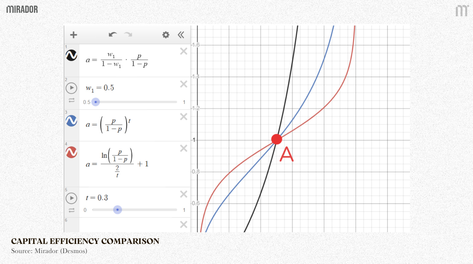
The slope of the curve shows how much the price changes for a given change in the asset proportion.
In simple terms, a flatter slope means the pool can absorb larger trades with smaller price impact, indicating higher capital efficiency.
From the graph, we can see that for the selected parameters (giving the same points of trading), the Notional AMM model achieves the highest capital efficiency.
Therefore, with the ability to customize AMM for each pool (by changing rateAnchor and rateScalar), Notional AMM was chosen by Pendle V2 as its inspired AMM model. This model will be discussed in a very detailed way in the following section.
CONCLUSION
In this first part of the series, we addressed the core challenge behind fixed-yield trading on-chain: how Principal Tokens (PTs), whose fair value deterministically converges to 1 at maturity, can be traded efficiently through an Automated Market Maker. By examining three AMM paradigms, we simply explained why Notional’s AMM architecture became the foundation for Pendle V2.
However, this overview only scratches the surface. The real sophistication of Pendle V2 lies not just in the pricing formula itself, but in how it is implemented on-chain, how trades update pool states, how implied yields are computed in real time, and how liquidity providers are protected as maturity approaches.
In Part 2, we will dive into the Pendle V2 AMM in detail, unpacking its on-chain mechanics, trade flow, state transitions, and the exact way fixed yields are expressed, traded, and settled within the protocol.
DISCLAIMER:
This article is intended as a conceptual and educational exploration of Automated Market Maker (AMM) designs for on-chain fixed yield trading. The focus of Part 1 is on economic intuition, pricing logic, and mathematical structure, rather than exhaustive smart contract implementation details.
Part 1 serves as a theoretical foundation for understanding why fixed yield instruments require specialized AMM architectures. A detailed examination of Pendle V2’s on-chain AMM design, trade flow, and state mechanics will be presented separately in Part 2.
Regarding this, such a brilliant breakdown of AMMs, thank u.