

PENDLE AMM - THE HIDDEN ENGINE OF YIELD TRADING – PART II: PENDLE V2 AMM DEEP DIVE
Understanding the working mechanism of Pendle V2 AMM via both the theory and reality on-chain

INTRODUCTION
Last week, we took a quick look at some potential AMMs for fixed-yield trading in the part 1 of Pendle AMM, including Constant Geometric model, YieldSpace’s and Notional’s.
In this Part 2, we will deeply dive into the AMM model behind Pendle V2 to explore the pros and cons of its pricing mechanism, together with our detailed mathematical explanation and swapping transaction via Pendle’s AMM in reality.
KEY TAKEAWAYS
This article is a detailed explanation of how Pendle V2 works via the following main sections:
Section 1: Understand the essence of Pendle V2 AMM’s pricing mechanism through the mathematical breakdown and Flash Swap mechanism
Section 2: Examine the strengths and weaknesses of Pendle V2 AMM
Section 3: Explore how Pendle V2 AMM works in practice through a swapping transaction on-chain
BEFORE WE BEGIN
Pendle V1 enabled trading PT and YT through two distinct liquidity pools, thereby causing capital fragmentation. To address this, Pendle’s new AMM was launched in V2, which only allows LPs to add PTs and the yield bearing token or SY tokens instead of YTs in V1.
These two tokens are closely correlated, with a high expectation of causing no impermanent loss for LPs. On top of this, PTs and YTs can be traded just inside a single pool of PT liquidity, via flash swaps mechanism (explained later), boosting capital efficiency.
Recognizing the pros of Notional’s AMM as proven in the previous section, Pendle V2 inherited this model and adapted for better efficiency.
Now let’s see how Pendle improves its AMM!
SECTION 1: THE CORE OF PENDLE V2 AMM - PRICING MECHANISM
Unlike other traditional AMMs like Uniswap or Curve, where AMM pricing is off spot price, Pendle AMM is based on yield rate (or implied rate).
The reason is that users trade PT and YT on Pendle with their expected implied APY (or trading yield, not trading the price).
Example:
Say a user predicts the implied APY of syrupUSDT will increase in the future, he can buy YT to expect a higher yield than the current one. And vice versa, if the implied APY is predicted to decrease in the future, he can buy PT to receive a higher fixed yield in case the implied APY truly goes down.
1/ Pricing mechanism
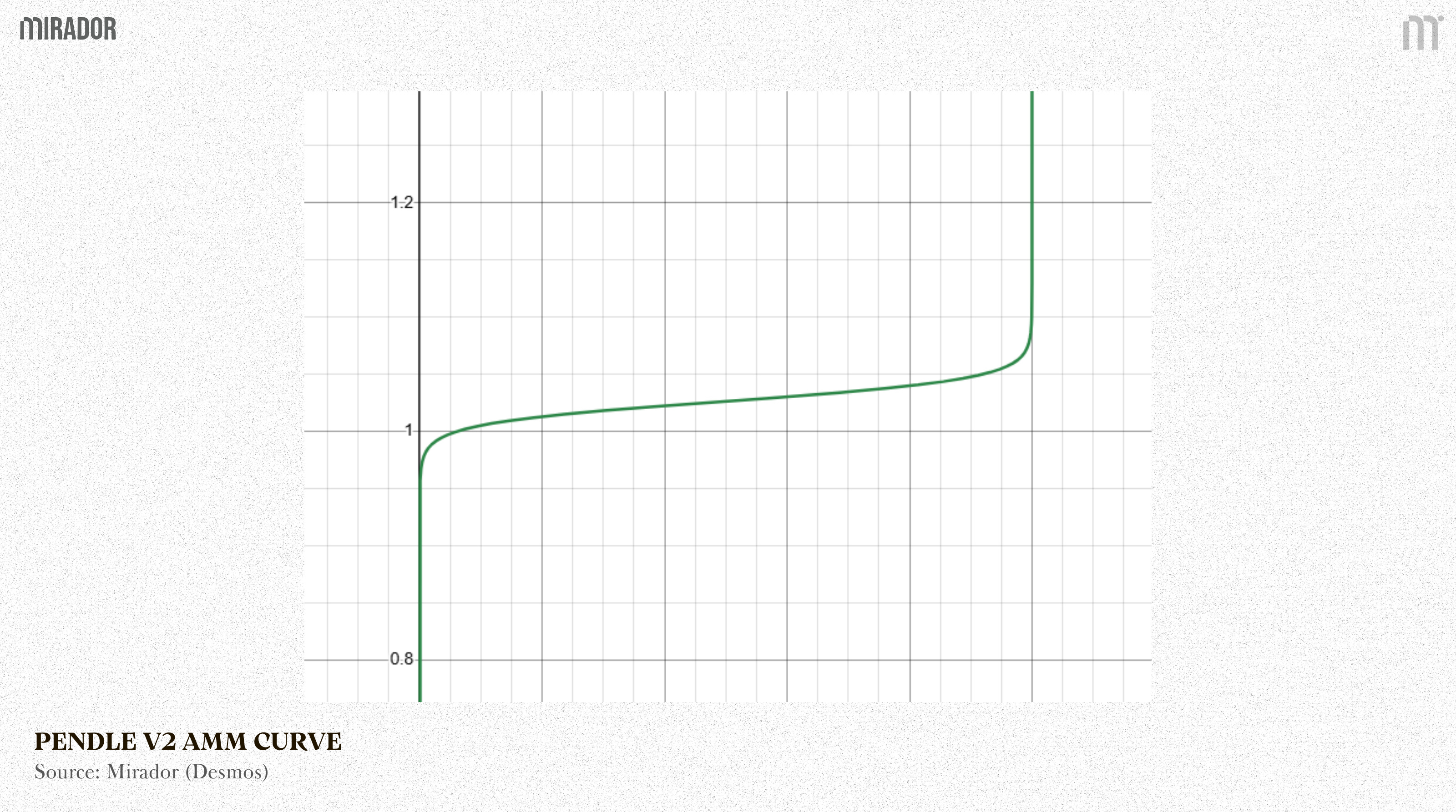
Pendle AMM is a logit curve (S-shaped curve).
This is the final exchange rate equation (or pricing formula) for the Pendle V2 AMM.
Where:
exchangeRate(t): the spot exchange rate of asset in PT (in case of no fee) at time t (exchangeRate(t) >=1 since 1 PT can be redeemed 1:1 at the maturity)
p(t): the proportion of PT in the market at time t [p(t)=n_pt/(n_pt+n_asset)]
rateScalar(t): a parameter used to adjust the capital efficiency (also known as the slope coefficient of the price curve, which adjusts for interest rate sensitivity)
rateAnchor(t): a parameter used to adjust the interest rate around which the trading will be the most capital efficient (also known as the anchor point of the curve, reflecting the interest rate around which it is “most stable”)
1.1/ Why a logarithm {ln[p/(1-p)]} appears in the pricing formula?
In Pendle, logit models the relationship between supply-demand PT and implied APY. Pendle’s AMM determines the exchangeRate, meaning the asset price in PT, reflecting the implied APY that the market “implicitly” prices.
Previous models (like Uniswap, YieldSpace) used power function or geometric mean, so:
Can’t simulate “PT → 1 at expiry” behavior.
Can’t adjust curvature depending on time or yield range.
Pendle chose the logit function because this S-shaped curve closely describes the actual supply and demand behavior of the yield market.
When p is close to 0 or 1, the slope is very steep (facing high slippage at both ends - similar to the case that the market is illiquid)
When p moves around 0.5, the slope is flatter, securing the efficient liquidity.
1.2/ How can Pendle ensure that the PT value can be redeemed 1:1 at the maturity?
The reason is behind two main parameters: rateScalar and rateAnchor.
A) RateScalar

One of the most important parameters in the pricing mechanism of Pendle AMM is the rateScalar.
According to Pendle docs, rateScalar(t) is a parameter used in calculating the exchangeRate at time t to adjust the capital efficiency.
Where:
scalarRoot: the base scalar rate, set by the pool owner
yearsToExpiry(t): the remaining period until the expiry date
Over time, when yearsToExpiry decreases, the rateScalar goes up and 1/rateScalar goes down.
When 1/rateScalar → 0, exchangeRate → rateAnchor
And what would happen next?
B) RateAnchor
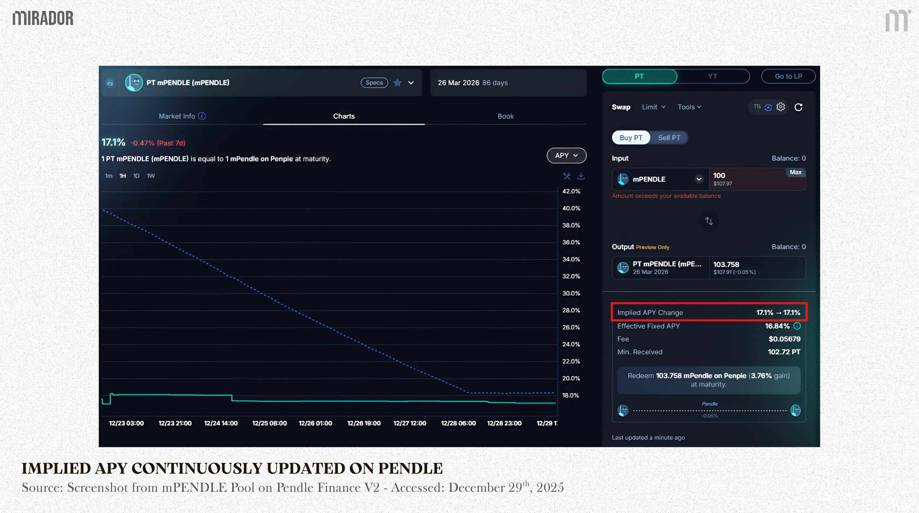
rateAnchor(t) is a parameter used to adjust the capital efficiency, anchored by a “continuity condition”. During operation, Pendle always updates this parameter such that the pre-trade implied APY at t is the same as the last implied APY in order to prevent arbitrage and manipulation.
rateAnchor formula:
When yearsToExpiry and 1/rateScalar → 0, rateAnchor(t) → lastImpliedRate^0→ 1
And exchangeRate → 1
As a result, PT prices on the AMM naturally converge to par as expiry nears.
In general, this rateScalar and rateAnchor help AMMs ensure that the PT price remains stable and converges to its original value as it nears maturity.
1.3/ Is there any difference between Pendle V2 AMM and Notional’s?
At its core, the pricing formula of these two models is totally the same. The only distinction lies in the changing of variables for easier complementation.
Because natural logarithms and exponents are easier to compute, Pendle introduced some changes in how these parameters are calculated on-chain, based on two factors:
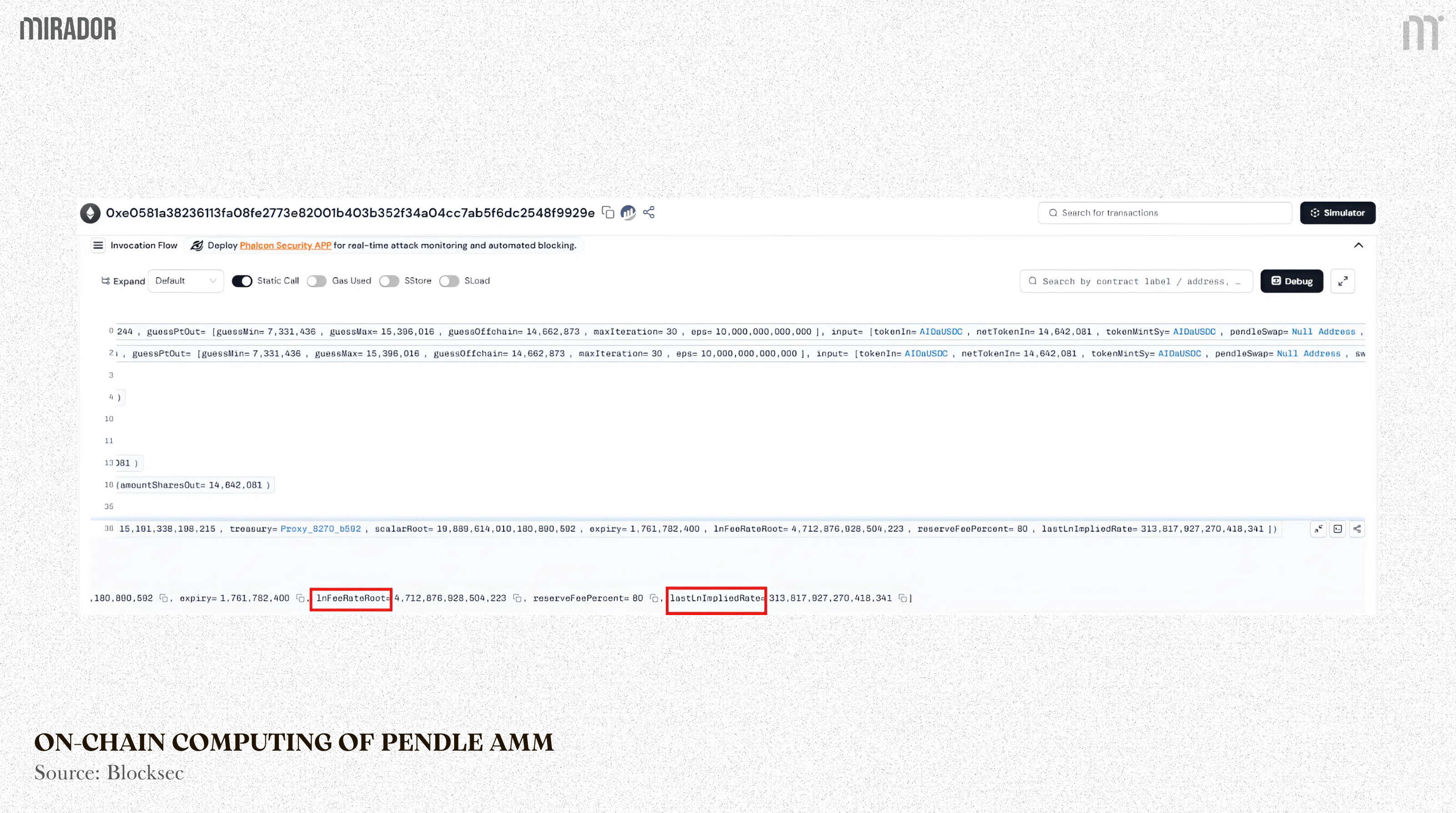
lnFeeRateRoot: logarithm of the base fee rate (protocol fee)
ln(lastImpliedRate): logarithm of the implied APY of the most recent trade.
You can see these two parameters in the real-time transaction below.
2/ Flash Swap Mechanism (Pseudo-AMM)
A liquidity pool in Pendle, in theory, has only two tokens: PT and SY (called PT/SY pool). So how can YT can be traded or swapped without a YT pool?
The secret is behind the Flash Swap mechanism, also known as Pseudo-AMM that allows users to both swap PT and YT using just a single pool.
Because PT and YT can be minted from and redeemed to its underlying SY tokens, the relationship among them is as follows:
Most importantly, YT price is inversely related to PT price.
Let’s see how this mechanism works on two distinct cases: selling & buying YT
2.1/ Selling YT
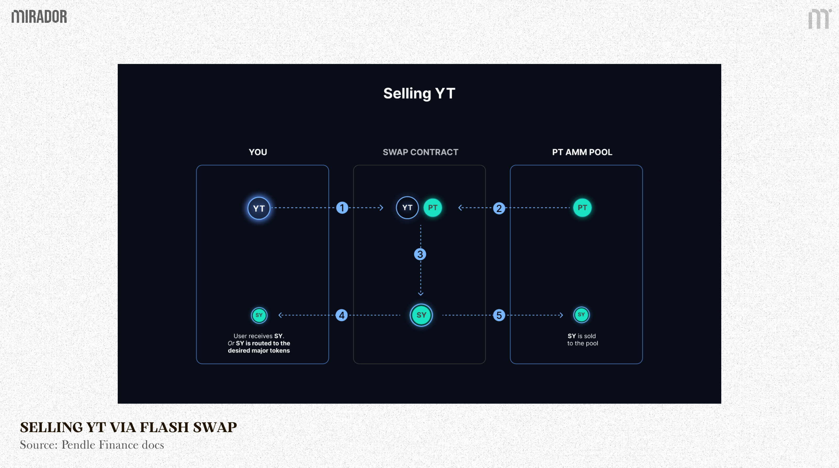
The selling YT flow is:
Trader sends YT into the swap contract to sell
Contract borrows an equivalent amount of PT from the liquidity pool
The YTs and PTs are used to redeem SY tokens
SY tokens are sent to the seller
A portion of the SY would be sold to the liquidity pool for PT to return the amount from step 2
For better simplicity:
Say Quinn wants to sell 10 YT-USDe in the PT/SY-USDe pool
Quinn sends 10 YT into the PT/SY pool for selling
Pendle creates 10 PT (virtual mint) for computing
Pendle integrates 10 PT and 10 YT → 10 SY
Assume at the current time 1 PT = 0.9 SY (prior to maturity)
Pendle swaps 9 SY → 10 PT. So there’s only 1 SY left
The contract will burn 10 virtual minted PT
The remaining 1 SY is the result of selling YT
→ Conclusion: Quinn sells 10 YT to receive 1 SY → 1 YT = 0.1 SY
→ Her profit is valued 1 SY
2.2/ Buying YT

The flow of buying YT is also the same as selling YT. Here’s the breakdown:
Trader sends SY into the swap contract to buy YT
Contract withdraws more SY from the liquidity pool
Mint PTs and YTs from all of the SY
Contract sends the equivalent YTs to the buyer
The PTs will be sold for SY to return the amount from step 2
SECTION 2: PENDLE V2 AMM – STRENGTHS AND WEAKNESSES
Now we will examine the pros and cons of Pendle V2 AMM model in each section below.
1/ The Strengths of Pendle V2 AMM
Adapted from Notional’s AMM, Pendle V2 pricing model is proven to go with the following advantages.
1.1/ Reducing complexity (cheaper gas cost and trading fee)
In the old model of V1, the pricing of PT/YT is complicated because:
PT, YT and SY lie in each distinct liquidity pool
The time to maturity needs to be computed, causing price volatility and difficulty in liquidity consuming.
→ The transaction cost was higher for traders.
As shared by TN Lee - co-founder of Pendle via an interview on Youtube, in Pendle V1, the user adoption is quite low since sometimes, the cost of one single transaction could reach up to thousands of dollars, which was extremely insane and impossible.
However, in V2:
PT/YT/SY are traded in a single pool, making PT ↔YT ↔ SY transactions smoother, cheaper, and simpler.
→ The gas cost was significantly decreased
1.2/ Liquidity Concentration - Greater Capital Efficiency
In V1, liquidity was fragmented across different pools. In order to tackle this problem, V2 was introduced with a new functionality called permissionlessness. This allows everyone to deploy liquidity pools on Pendle, as well as allows them to set the effective liquidity range of their own pools.
For example, if you predict that stETH’s APY tends to fluctuate in the range of 0.5-6%, you can customize your pool by concentrating liquidity within this range only, supporting much larger trade sizes at a smaller slippage.
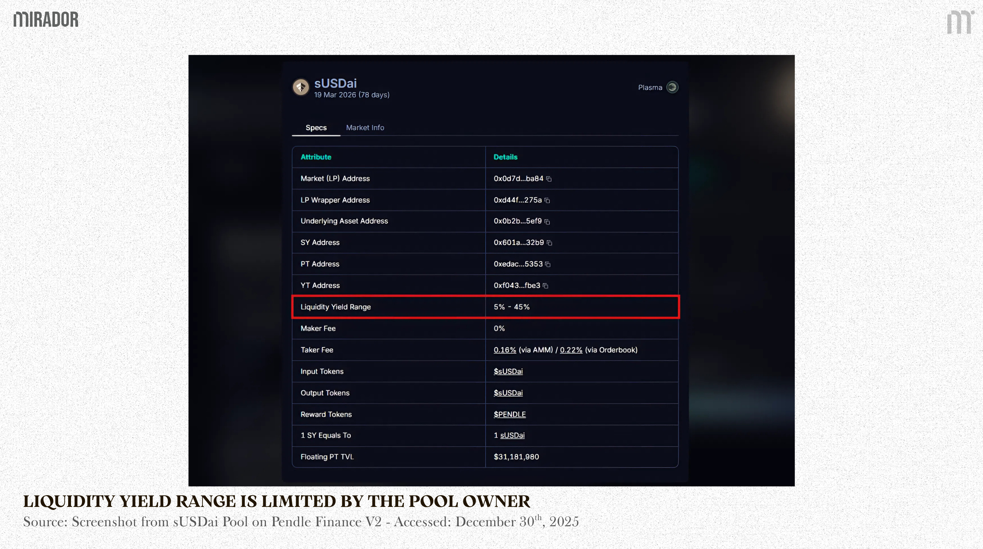
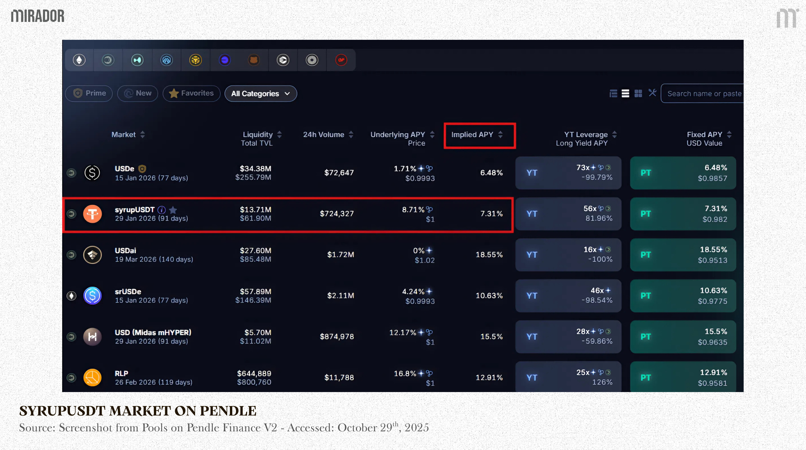
As seen in the sUSDai market above, the liquidity yield range where the pool is active ranges from 5% to 45%.
It means that the majority of liquidity will focus on this yield range only (beyond 45%, buying YT/selling PT might not be possible), boosting the capital efficiency. This is also a good way to improve the actual accrued transaction fee for LPs.
1.3/ Reduced Impermanent Loss (IL)
Different from other AMMs like Curve or Uniswap, where the trading is around the asset’s spot price, the core of Pendle is for yield trading. So in most cases, PT is traded within a specific yield range that does not fluctuate as much as an asset’s spot price.
Assume that Euler’s USDC lending rate tends to fluctuate between 0%-12%, and PT will be accordingly traded within that APY range.
This ensures that the IL is minimal at any time since PT price will not deviate too far since liquidity is provided.
Moreover, if liquidity is provided until maturity, an LP’s position will be like fully holding the underlying asset since PT naturally approaches 1:1 the underlying asset thanks to the mechanism of AMM (as proven above).
2/ The Risks of Pendle V2 AMM
The risk of Pendle V2 AMM mainly revolves around two main aspects: liquidity risk and other risks (dependent factors).
2.1/ Liquidity risk
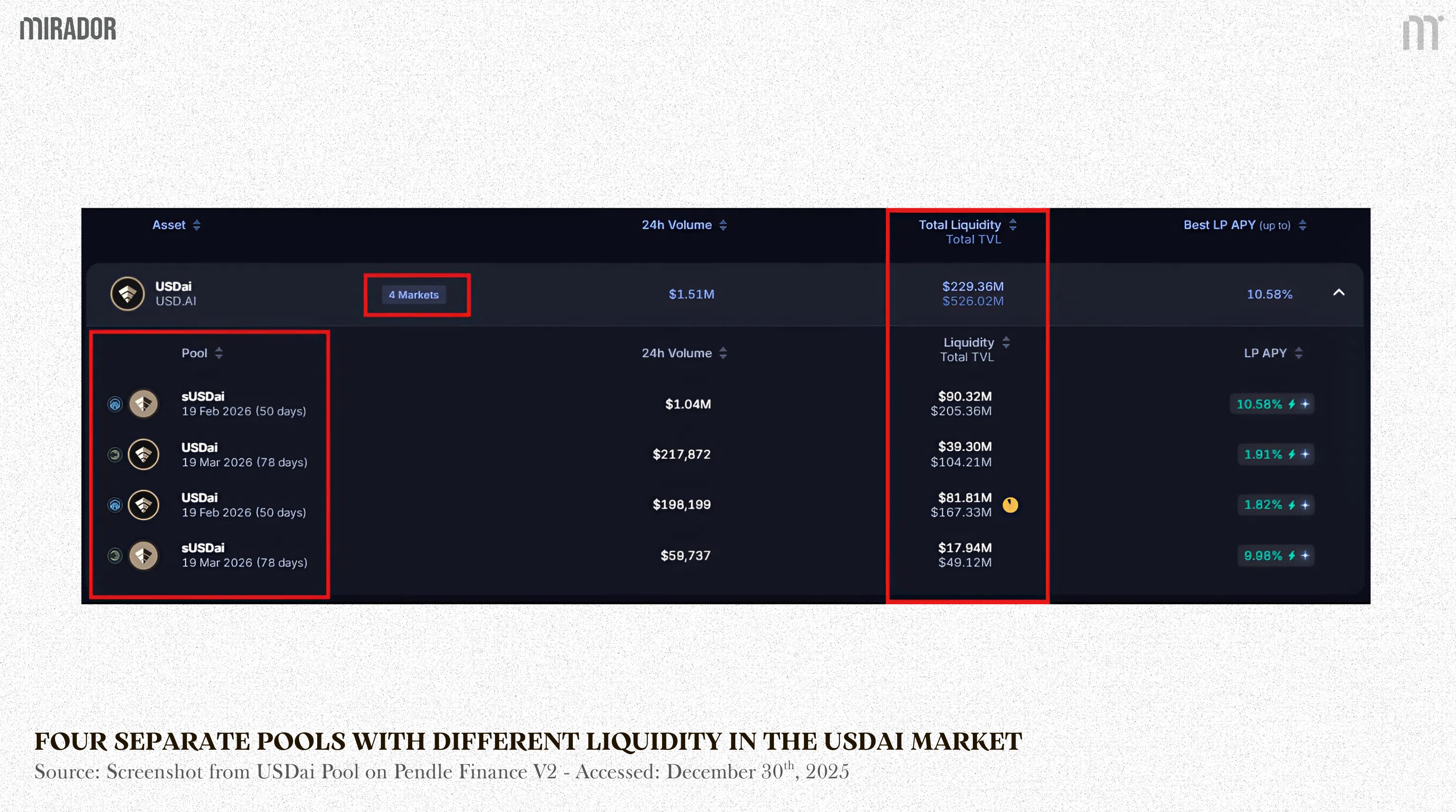
A) Liquidity fragmentation by maturity
In reality, Pendle V2 AMM was born to deal with liquidity fragmentation in its early version, but has not been completely resolved.
Each token with different time to expiry (like 1st Jan, 2026; 1st Jun, 2026…) is a separate pool as you can see in the USDai pools below.
When the old maturity expires, liquidity must gradually shift to the new maturity, reducing the overall liquidity depth, especially in the long term.
B) Impermanent loss still exists
Because of the freedom in pool creation, theoretically, LP on Pendle V2 still faces impermanent loss, especially in the pool configured with a wide yield range.
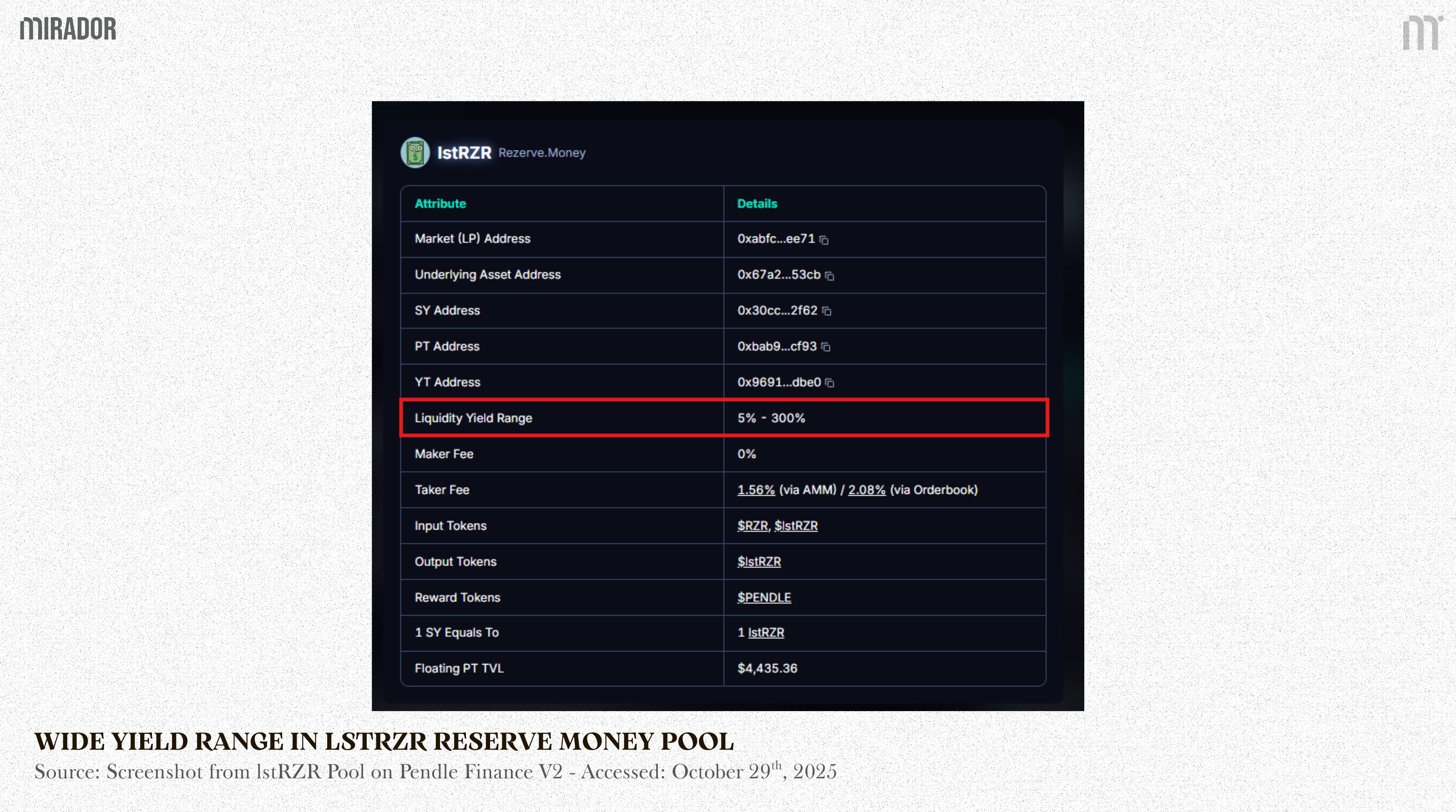
Example:
The lstRZR Reserve Money pool is set with a super wide liquidity yield range (max 300%). It means the APY can vary strongly in this range, which may cause IL for LPs. Therefore, LPs should check out this parameter carefully before deciding to add liquidity.
2.2/ Other risks from dependent factors
To be honest, as of now, Pendle’s new AMM is still proven to face no critical risks. The risk of this model mainly comes from other dependent factors that theoretically may happen.
A) Smart contract complexity
Pendle V2 uses multiple logic layers: Tokenization (PT/YT minting), SY conversion layer, AMM pricing layer (logit curve, rateScalar/rateAnchor updates). So the smart contract system is very complex, which may entail the higher risk of logic bugs or rounding errors.
B) SY tokens
SY can be any yield-bearing token (stETH, aUSDC, cDAI,…). If the underlying protocol meets a critical problem (smart contract hack, depeg, etc.) → PT and YT both lose value.
For example: If Morpho has a problem with USDC→ the entire PT-USDC pool may lose the ability to redeem.
SECTION 3: USE-CASE - SWAPPING VIA PENDLE V2 AMM
In this section, we will try working out a real-time swapping transaction to see how Pendle V2 AMM works and how PT can be redeemed at 1:1 for the accounting asset at maturity.
For better illustration, we deliberately take the AIDaUSDC pool, which is really soon to expire, only one day left until maturity (30 Oct 2025), as an example. Though until now, this pool has expired but this doesn’t affect our calculations.

On Pendle UI, if I want to swap 14.64 AIDaUSDC, the amount of output PT that users are expected to receive is 14.6594 PTs. This is all via AMM of Pendle V2. So now we will explore how Pendle’s AMM can compute the swapping transaction.
We found a swap-token-for-PT transaction (or buying PT) on
. Below is the market information of this pool that we tracked (numbers have been adjusted for easier understanding based on decimal figures):
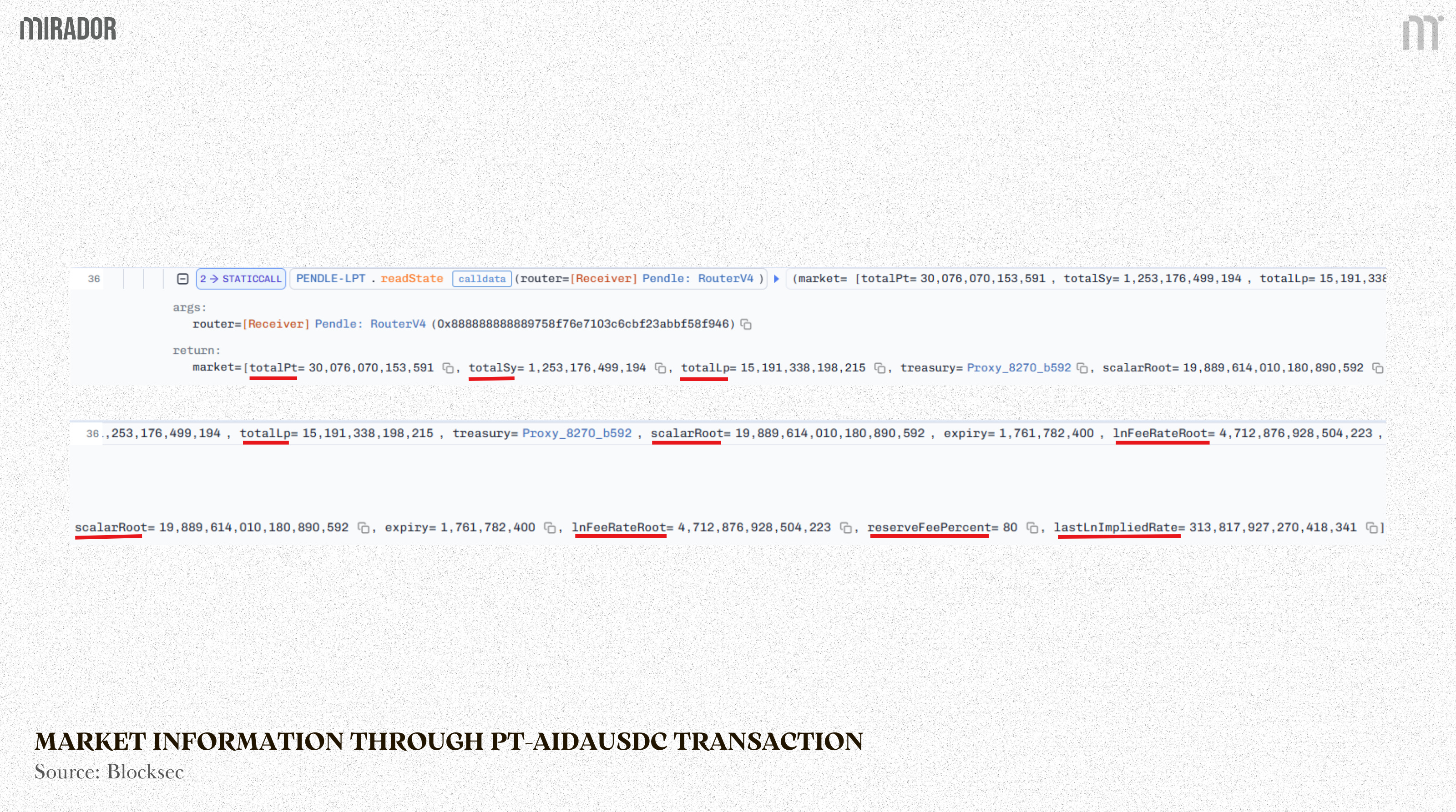
totalPT = n_pt = 30,076,070 (total PT-AIDaUSDC available in the pool)
totalSY = n_sy =1,253,176 (total SY-AIDaUSDC available in the pool)
scalarRoot = 19.889 (set by the pool owner)
lnFeeRateRoot = 0.004712 (Base logarithmic fee rate - however, in this case, we will simplify this problem by assuming there’s no fee at all in swapping since the actual fee is quite trivial. So just pretend this number never existed)
lastLnImpliedRate = 0.313 (Logarithm of last implied Rate, as seen in the UI, last Implied Rate/APY is about 36.86%)
d_asset = 14.64 (The amount of input asset (AIDaUSDC) is 14.64)
The question: d_pt = ? (how many output tokens (PT) would a user receive?)
SOLUTION:
Remember that the Pendle V2 AMM is based on this formula:
Now let’s solve it together!
First, we need to find out the rateScalar parameter. Now we have:
To find out the numerator, we need to understand about p(t). As written in the Pendle docs:
Where:
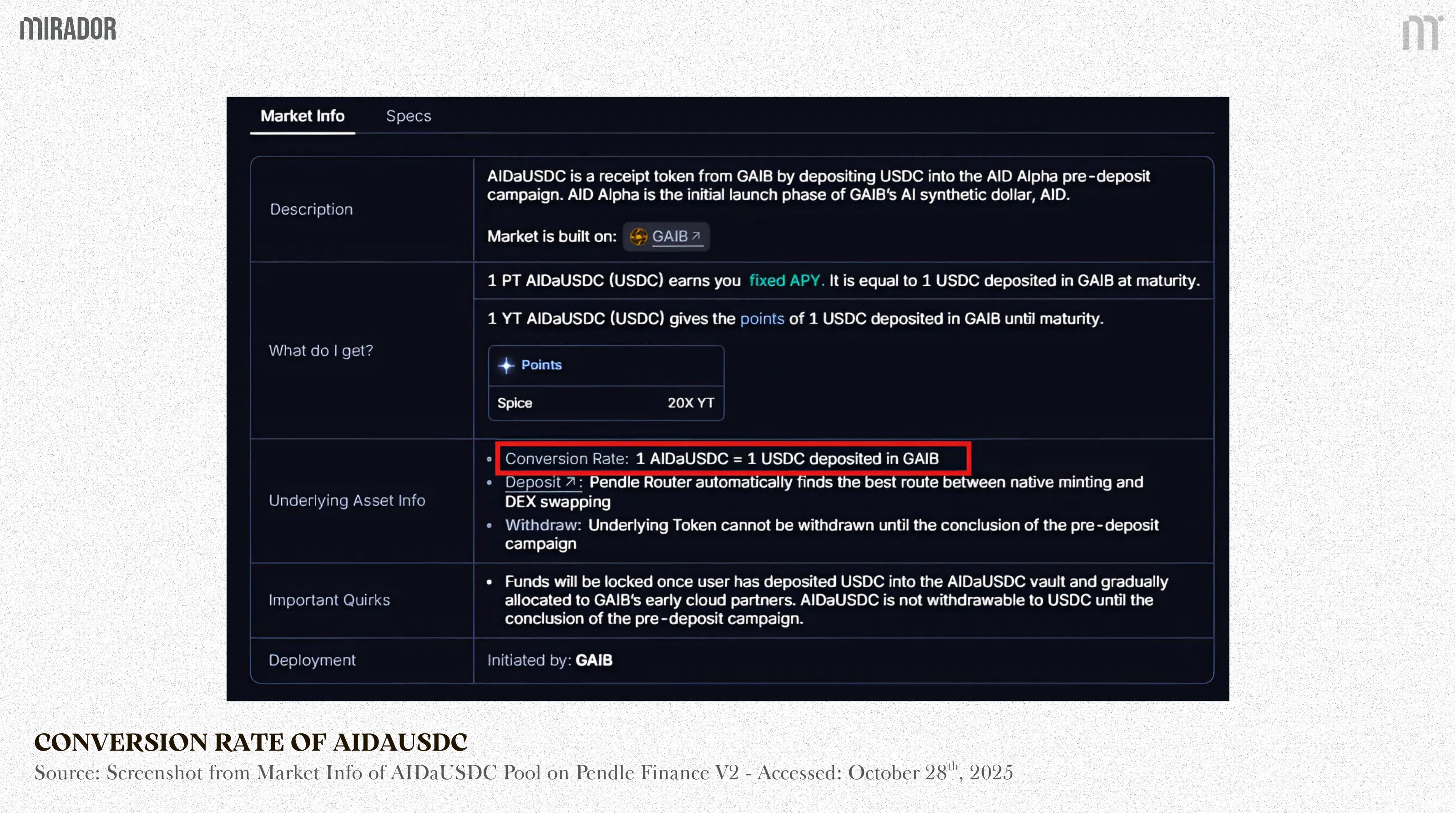
In this case, 1 AIDaUSDC = 1 USDC deposited in GAIB
→ syExchangeRate = 1 → n_asset = n_sy = 1,253,176
Hence:
Since this pool has only one day left till the maturity, the amount of PT occupies most of the pool (about 96% - which is also the PT share cap in the pool that Pendle sets to ensure that YT is still sufficiently available for trade)
The last attempt is to find out rateAnchor, which is a parameter used to adjust the interest rate where the trading will be the most capital efficient. Here’s how to calculate it:
Breaking down every steps and this leads to:
Note that:
The lastLnImpliedRate in the contract is 0.313 → last Implied Rate = e^0.313 ≈1.3675
This number doesn’t mean the implied APY would be 136.75%, but instead the return rate is 36.75% (which might be slightly different from the implied APY on Pendle UI (36.86%) due to small errors in mathematical calculation). For other examples, if an interest rate per year is 5%, the return rate would be 1.05%).
Now let’s move to the last step, calculating the Exchange Rate to find out how many PTs we would receive by theory (in case of no fee).
exchangeRatenoFee=ln(p1−p)rateScalar+rateAnchor≈0.000438018+1.000419884≈1.000857902
With the above exchange rate, theoretically the amount of PT the swapper would receive is:
dPT(noFee)=exchangeRatenoFee×dasset=1.000857902×14.64≈14.652564 PT
This number is quite close to the amount of output PT as seen on Pendle UI (14.6594 PT - which was included a small fee and slightly differs from the theoretical output number due to small error in calculation).
In short, with 14.64 input tokens (AIDaUSDC), we will receive a rather equivalent amount of output tokens (~14.65 PT). And when this pool’s matured, your PT-AIDaUSDC could be redeemed at 1:1 for the accounting asset (AIDaUSDC).
CONCLUSION
Pendle V2 marks a major step forward in AMM design for yield tokenization. While Pendle V1 relied on a constant geometric model and required separate liquidity pools for PTs and YTs, the new Pendle V2 AMM resolves these inefficiencies through allowing both PT and YT trading within the same liquidity structure.
Ultimately, Pendle V2 transforms its AMM from a simple token swap mechanism into a sophisticated yield trading infrastructure, one that optimizes liquidity, reduces risk for trading, and unlocks a more efficient market for tokenized yields.