


INTRODUCTION
Liquidation is the safety mechanism that keeps a lending protocol solvent. For borrowers, it is the moment collateral is forcibly sold and the loss becomes permanent.
Aave V3 relied on a cap based liquidation design, using hard thresholds and fixed incentive parameters to keep execution simple and reliable on the EVM. The tradeoff is that the outcome can be coarse. A position that is only slightly unsafe can be liquidated in a size that is much larger than what is needed to restore safety, and fixed incentives can concentrate MEV competition at the liquidation boundary.
Aave V4 proposes a different approach. It replaces static caps with a Target Health Factor solver that sizes repayment to a chosen safety baseline, and it replaces fixed incentives with a state based bonus curve that adapts as risk deepens.
This raises two practical questions for borrowers and liquidators.
Why does Aave V3 often liquidate more collateral than seems necessary for small breaches?
Does Aave V4 actually make liquidation more proportional, and how does it change liquidator competition and MEV dynamics?
This article answers these questions by reconstructing the exact sizing and incentive mechanics, then validating the key behaviors using empirical Aave V3 on chain liquidation data.
KEY TAKEAWAYS
In this article, we examine Aave liquidation mechanics in three parts.
Section A: Why cap based sizing in Aave V3 leads to overshoot, especially near the threshold
Section B: How Target Health Factor sizing in V4 mathematically enforces a chosen post liquidation safety baseline
Section C: How the state based bonus curve creates a Dead Zone and a Race Band, reshaping liquidator incentives and shifting MEV from a single trigger point to a competitive band
A/ WHY AAVE V3 LIQUIDATES MORE ASSETS THAN NECESSARY?
1. The Core Issue: Liquidation as Debt Recovery, Not Punishment
This section is a sizing question: when a position becomes liquidatable, how much debt should be repaid in the liquidation transaction ?
Aave V3 does not compute the minimal repayment needed to restore a position to a chosen safety buffer. Instead, it sets an upper bound on repay size, the Close Factor. In short, V3 provides a cap, not a target based solver.
Because the Health Factor (H) is continuous, a position at H just below 1 is only slightly unsafe, while a position at much lower H is deeply unsafe. A cap based rule does not scale smoothly with this risk depth. Within a given region, the cap is the same, and liquidators have a direct incentive to repay close to the maximum allowed size to maximize profit.
This is the core mechanism behind over liquidation in V3: post liquidation safety is not explicitly targeted. It is an emergent outcome of a coarse repay cap, profit maximizing liquidator behavior, and a liquidation bonus that scales collateral seizure with repay size.
2. The Mathematical Flaw of a Static Rule
2.1. State Variables and the Meaning of H < 1
To demonstrate why this “one size fits all” rule is inefficient, we define the core state variables (calculated in USD):
D : Total Debt.
V : Raw Collateral Value.
c : Liquidation Threshold (the risk parameter of the asset).
C : Eligible Collateral, where: C = c×V
H : Health Factor, the ultimate safety metric.(this is not calculated in USD)
The Health Factor is calculated as:
A position becomes eligible for liquidation when H < 1 . Economically, this means the risk adjusted collateral value C is no longer sufficient to cover the debt under the protocol’s risk rules.
2.2. Close Factor in Aave V3 Is Piecewise Constant, Not Truly Fixed
Aave V3 does not apply a single fixed close factor in all states. Instead, it uses a piecewise rule that still behaves like a static cap within each region.
Up to 50 percent of total debt can be liquidated when health factor is above 0.95 and both collateral value and debt value are at least 2000 USD each.
Up to 100 percent of debt can be liquidated when health factor is 0.95 or below, or when either collateral value or debt value is below 2000 USD.
So the execution rule is still a cap based approach:
where f is 0.5 in the normal region and can jump to 1.0 in the severe risk or dust region.
This matters for the argument. The over liquidation problem is most visible in the near threshold region, roughly 0,95<H<1 , where the cap can still be very large relative to what is minimally required to restore safety.
2.3. Why a Cap Creates Overshoot
Aave V3 does not compute the minimal repay amount required to reach a target safety level. It only sets an upper bound. In most profitable scenarios, liquidators rationally choose to liquidate as much as the cap allows, because profit scales with size.
To see the mechanical effect, write the post liquidation health factor for a simplified single collateral single debt position. Let b be the liquidation bonus. If the liquidator repays R , then collateral seized is approximately (1+b)R in USD terms, and the post state becomes
This formula shows why sizing matters. As R increases, debt decreases, but collateral also decreases and it decreases faster than debt because of the bonus term.
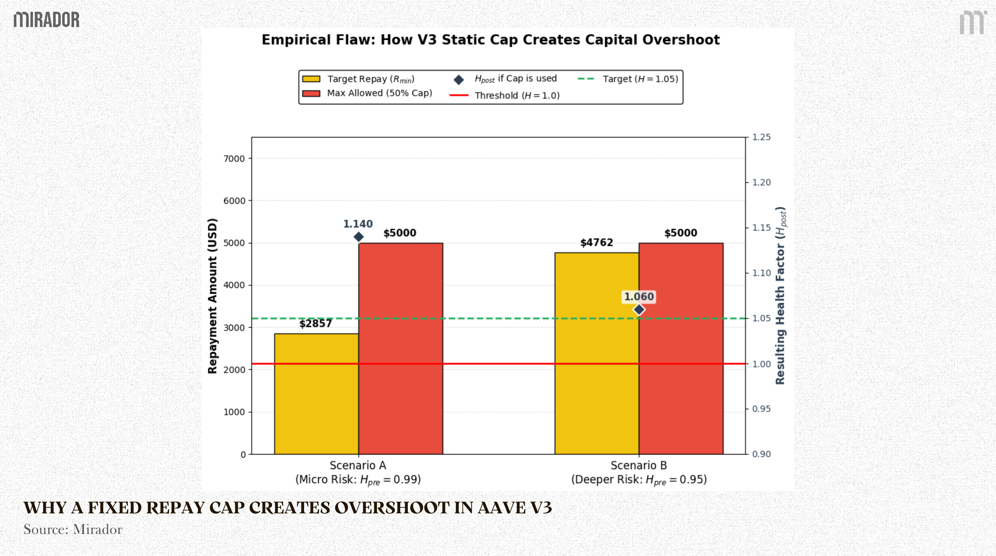
This chart compares two repay sizes for the same position state.
The yellow bar is the minimum repay needed to restore the position to a reasonable safety buffer (𝐻=1.05).
The red bar is the maximum repay allowed under the V3 50% close factor cap.
The diamond marker shows the resulting post liquidation health factor (𝐻𝑝𝑜𝑠𝑡) if the liquidator uses the cap.
Key takeaway: when the position is only slightly unsafe (Scenario A), the cap still permits a large repay, pushing (𝐻𝑝𝑜𝑠𝑡) well above the target buffer (overshoot). That higher buffer may reduce re liquidation risk, but it comes at a clear borrower cost: more debt is repaid and more collateral is seized than is strictly needed to restore safety.
3. Why V3 Used a Cap Based Model
3.1. Why a Simple Cap Worked Well on Ethereum Mainnet
Aave V3 was designed for a world where Ethereum mainnet transactions could be expensive and unreliable during market stress. In those moments, the protocol needs liquidations to execute quickly and predictably.
A close factor cap fits that requirement because it is extremely simple to compute. It only needs a few basic arithmetic operations.
Take the user’s total debt D
Multiply by a constant f
Get the maximum repay size Rcap=f×D
This is what people mean by O(1) . It does not mean “better” or “more fair”. It only means the computation is constant and small. No matter how complex the position is, the contract does roughly the same tiny amount of work.
Important clarification: O(1) explains why a constant cap is attractive, but it does not explain why the cap is 50%. Any constant cap, 30%, 50%, 70%, is still O(1) . The exact number is a design trade-off.
Higher cap: removes risk faster, fewer steps, better for solvency in fast crashes
Lower cap: reduces borrower loss from overshoot, but may require more repeated liquidations
The protocol also needs liquidators to show up, which pushes incentives toward simple, reliable execution
So the real reason V3 used a cap based design is reliability under stress, not mathematical necessity.
3.2. Why the Constraints Became Less Binding Over Time
Later, the environment changed in two practical ways.
First, more user activity moved to Layer 2 systems. Many L2 networks have lower fees and higher throughput than mainnet, which makes more complex on chain logic less risky to run in practice.
Second, the Dencun upgrade and EIP 4844 reduced the cost of sending rollup data to Ethereum using blobs. That lowered costs for many rollup transactions and made it easier for protocols to design richer execution logic in L2 environments.
The key point is not that computation becomes free. The key point is that the original constraints that strongly favored ultra simple liquidation logic became less severe. When costs and execution risk drop, a protocol can shift from “always do the simplest thing” toward “do the more accurate thing”, such as dynamically sizing the repay amount to hit a chosen safety target.
This is the design space Aave V4 is trying to use: replace coarse caps with a target driven mechanism, while keeping liquidations reliable enough that liquidators still participate during stress.
Example : How Alice Loses Capital
We can quantify this capital destruction through a step -by -step calculation of a minor risk scenario.
Initial state for Alice:
Debt (D): 10,000 USD
Collateral (V): 13,000 USD
Liquidation Threshold (c): 0.80
Close Factor (f): 0.50
Liquidation penalty: 0.05 (5%)
Step 1: The Risk Trigger
The market price drops slightly, reducing V to 12,250 USD.
Observation: Alice is just barely below the 1.0 threshold. She only needs to repay a tiny fraction of her debt to become safe again.
Step 2: The V3 Execution
Instead of calculating what Alice actually needs, the liquidator applies the maximum 50 percent Close Factor rule to maximize their own profit:
Debt repaid (R): 10,000×0,50 = 5,000 USD
Collateral seized from Alice (including the 5 percent bonus): 5,250 USD.
Step 3: The Overshoot
We calculate the ledger state post liquidation:
New Debt (D): 5,000 USD.
New Collateral (V): 7,000 USD.
New Eligible Collateral (c): 7,000 × 0,80=5,600 USD
The new Health Factor is:

The key point is not that a higher post liquidation health factor is always bad. A buffer above 1.0 can be desirable, especially for volatile collateral, because it reduces the chance of immediate re liquidation. The issue in Aave V3 is that this buffer is not explicitly targeted by the protocol. It emerges mechanically from a coarse close factor cap and profit maximizing liquidator behavior. In Alice’s case, repaying the full 50% pushes the position from H=0.98 to H=1.12, which may be a larger buffer than necessary for a marginal breach, and therefore increases collateral sold and the liquidation penalty paid.
4. Empirical Evidence from On-chain Data
To test whether overshoot is a rare edge case or a recurring pattern, we analyze liquidation events on Aave V3 Ethereum using Dune Analytics. The chart below compares the Health Factor immediately before and immediately after each liquidation event.
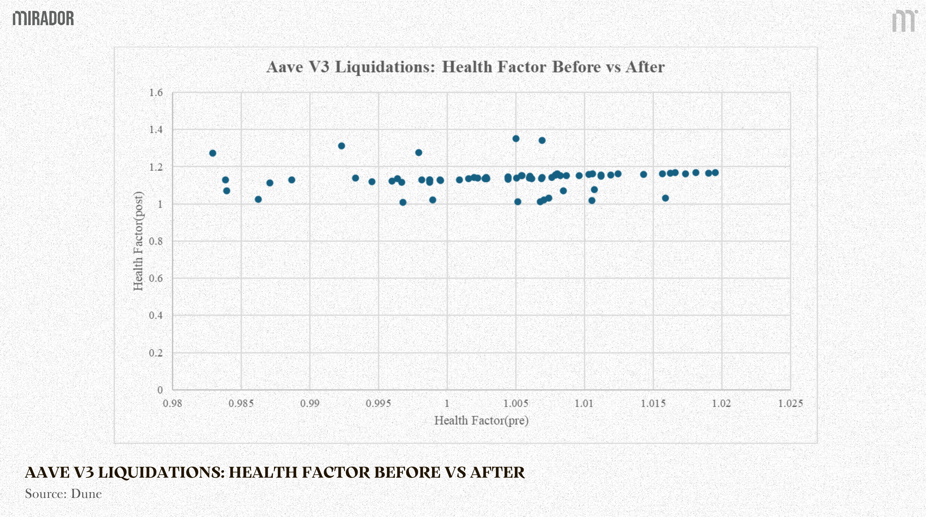
Horizontal Axis (X): Health Factor before liquidation (Hpre).
Vertical Axis (Y): Health Factor after liquidation (Hpost).
Interpreting the plot is straightforward. Points near Hpre≈0.99 represent positions that were only slightly below the liquidation threshold. If liquidation sizing were tightly calibrated, we would expect many of these points to land just above 1.0 after liquidation. Instead, a visible share of them jump to much higher post liquidation health factors, with many exceeding 1.12. In other words, the data suggests that a meaningful number of near threshold liquidations result in a post state that is substantially safer than the minimum required to exit liquidation.
This pattern is consistent with the mechanism described earlier: within the close factor capped region, liquidators have an incentive to repay close to the maximum allowed amount, and the liquidation bonus causes collateral seizure to scale with repay size. The result is a larger buffer, but also higher borrower cost, especially when the initial breach was smal
A static cap is a reasonable engineering choice when reliability under congestion is the primary constraint, but it also makes liquidation outcomes coarse. The evidence above does not imply that every overshoot is bad. In volatile markets, a higher buffer can reduce the chance of immediate re liquidation. The core takeaway is more specific: in Aave V3, the post liquidation buffer is not explicitly chosen by design for each risk state. It emerges from a fixed cap plus profit maximizing execution.
This is the design motivation for a dynamic liquidation engine in Aave V4. Instead of relying on static constants to indirectly produce a safety buffer, V4 aims to compute repayment sizes that target a chosen post liquidation health factor, and then adjust incentives so liquidators still participate reliably across different risk states.
B/ THE V4 SOLUTION: TARGET HEALTH FACTOR SIZING
Part A showed that Aave V3 is cap based: it defines a maximum repay size per liquidation, but it does not compute the repay size needed to reach a specific post liquidation safety buffer. This creates room for overshoot, especially when the position is only slightly below the threshold.
The chart below reframes the same liquidation events through a counterfactual question: for each real Aave V3 liquidation, what repay amount would Aave V4 have requested if the position were liquidated using a Target Health Factor solver. Each dot is one on chain V3 liquidation event.
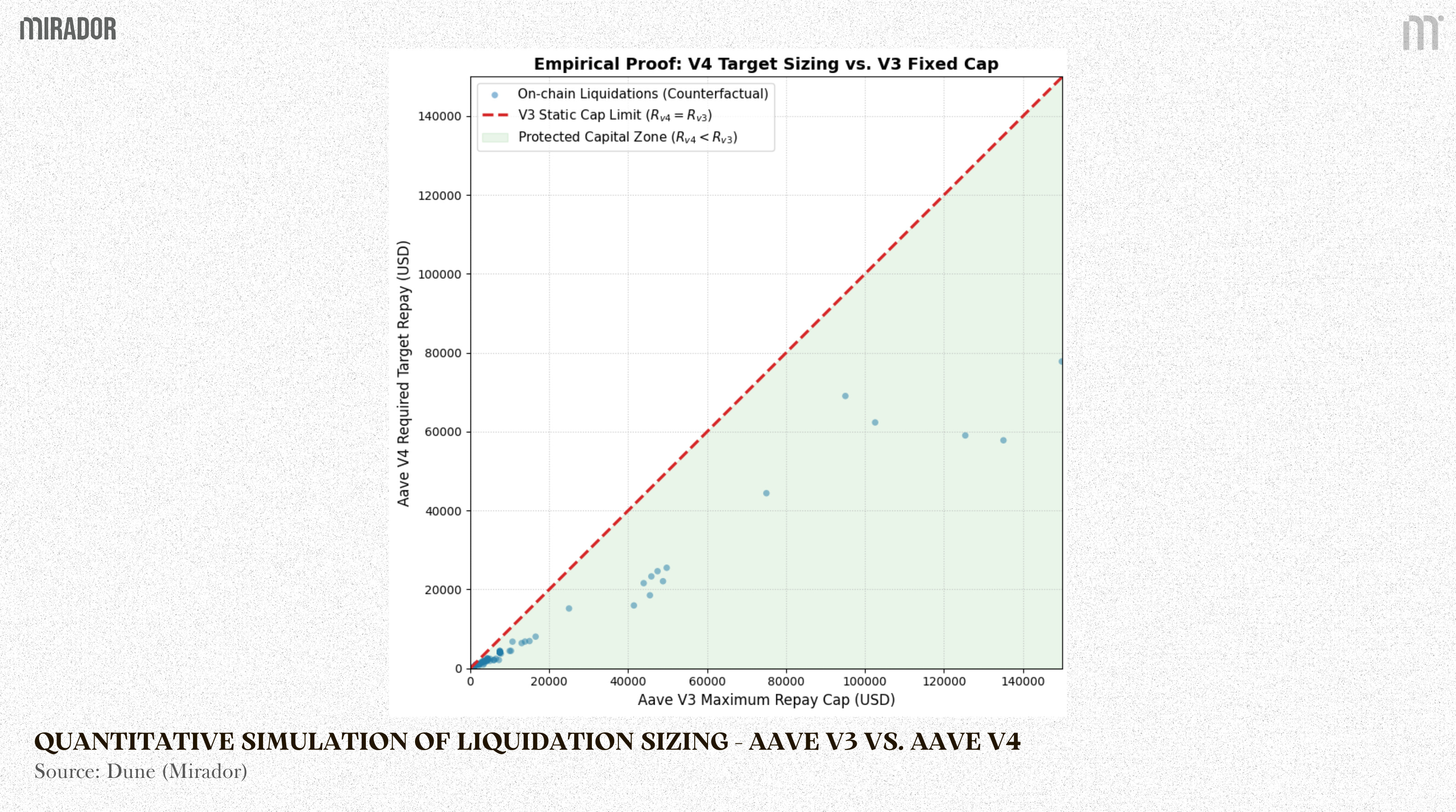
Horizontal axis X: the maximum repay cap that Aave V3 would allow for that specific event state.
Vertical axis Y: the repay amount required by a V4 style target solver to restore the position to the chosen target safety level.
Points below the diagonal line indicate cases where the target solver would repay less debt than the V3 cap permits. In those cases, the required collateral seizure would typically be smaller, implying less borrower capital sold than a cap maximization outcome. In our sample, the points cluster below the diagonal, consistent with the claim that target based sizing can reduce overshoot near the threshold.
To understand why this happens, we now unpack the V4 solver itself. The core mechanism is the function _calculateDebtToTargetHealthFactor, which computes the debt to repay so the post liquidation Health Factor is steered toward a predefined target.
1. The State Variables
To establish the equation, we define a loan position with all parameters normalized to USD ( expect Health Factor) :
· D: Total current debt.
· V: Raw collateral value.
· τ: Liquidation Threshold. This is the risk parameter of the asset used to calculate safety (e.g., 0.80). It is distinct from the Loan to Value ratio used when initially opening a position.
· C: Eligible collateral value, where C=τ.V
· H: Initial Health Factor, where H = C/D. The position is eligible for liquidation when H<1,0.
· T: Target Health Factor configured by the system (e.g., 1.05). The algorithm must find a way to return H to this exact T baseline.
· b: Liquidation Bonus. While this bonus varies depending on risk depth, during the sizing step of a specific execution, this bonus is locked based on the initial state (H_pre) and enters the equation as a constant: b=b(H_pre).
· R: The exact Repay Amount (the target variable).
When a liquidator repays a debt amount R, they receive the equivalent raw collateral plus the bonus: R×(1+b).
Consequently, the eligible collateral (C) of the position will decrease by a corresponding amount: τ×R×(1+b).
The post liquidation ledger state of the position becomes:
· New Debt (D): D-R
· New Eligible Collateral (C’): C-τ.R.(1+b).
· New Health Factor (H’): (C^’)/(D^’)
2. Deriving the Repay Formula (R)
The system must solve the equation so that the new Health Factor perfectly matches the target (H’=T).
We apply algebraic transformation to isolate R:
The core formula executed within the Solidity codebase is:
The Mathematical Existence Constraint:
For this function to return a valid result (a positive repay amount), the denominator must be strictly positive:
This constraint is not just a technical requirement for division. It has a practical meaning. The term τ×(1+b) captures the effective haircut on collateral once the liquidation bonus is included. If governance sets the target T too low relative to this haircut, the solver can return an invalid or negative repay amount, or the transaction may revert. From a system design perspective, Aave governance must configure the target T and the maximum bonus limits so this inequality holds across supported collateral types and market conditions
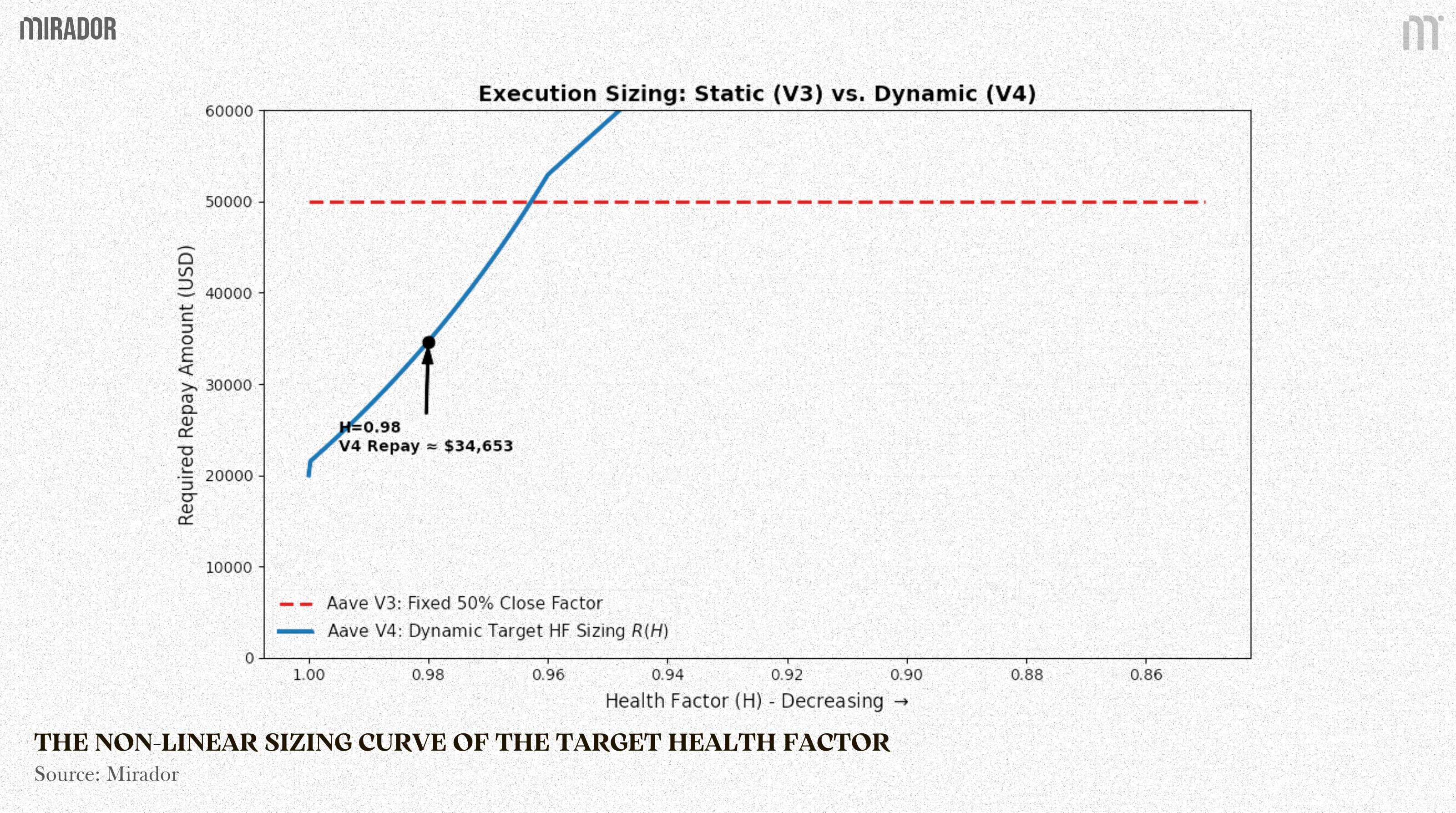
The chart compares two sizing rules. The red dashed line is the V3 repay cap in the 50% close factor regime. The blue curve is the V4 target solver, the repay amount needed to reach T=H’ at each starting health factor H .
If the blue curve is below the red line, V4 would repay less than the V3 cap, so the borrower typically loses less collateral in near threshold liquidations.
Does target sizing create liquidation cascades?
A natural concern is repeated liquidations during a prolonged drawdown. If collateral prices keep falling, a position can be liquidated back to T, then quickly drop below 1 again and be liquidated again. This is a real trade-off, but it should be framed as frequency versus severity. A cap based system tends to produce fewer but harsher liquidations, while a target based system can produce more frequent but smaller liquidations by avoiding cap sized overshoot. Governance mitigates churn by choosing a target T that provides a meaningful buffer above 1, balancing the risk of immediate re liquidation against the borrower cost per event.
3. Safety Checks: Repay Clamp and the Dust Rule
The algebraic result R is referred to in the codebase as _debtToTarget. However, the smart contract does not execute this raw number immediately. It must route the value through two layers of boundary checks to ensure ledger safety.
Layer 1: The Execution Clamp
The actual executed liquidation volume (R_actual) is bounded by the total outstanding debt and the amount the liquidator is willing to cover:
Meaning:
debtToTarget is the solver output, what the math would like to repay
debtToCover is the liquidator’s chosen maximum, how much they are willing to repay in this call
debtReserveBalance is the user’s actual outstanding debt in the repaid reserve, the real debt balance the contract can close, including interest accrual and rounding effects
Layer 2: The Dust Debt Exception
The Target HF rule is the default calculation method. However, it is constrained by the execution economics of the Ethereum network, specifically Gas fees.
If the remaining debt after liquidation (D -R_actual ) is too small (strictly less than a constant like DUST_LIQUIDATION_THRESHOLD, e.g., 1,000 USD), the future Gas cost to liquidate this tiny remainder will exceed the bonus value. No bot will execute it, leaving the protocol with toxic bad debt.
To prevent this, the codebase establishes an exception rule: If
D - R_actual<1,000 USD, the protocol abandons the Target HF formula. It allows the liquidator to repay 100 percent of the outstanding debt to completely wipe the position clean.
This design is smart for two reasons:
It protects the protocol by ensuring the liquidation result is actually cleanable in practice, not just correct on paper. Dust is a real failure mode because bots follow economics, not intent.
It also protects borrowers in the common case by enforcing a repay amount closer to what is needed for safety, instead of letting liquidators automatically push to a large cap.
The trade-off is that the dust path prioritizes system hygiene over borrower smoothness. When dust would be created, the protocol is willing to be more aggressive and close the position fully.
4. Execution Trace and V3 Comparison
To prove the precision of the function, we run a step -by -step execution trace.
Initial position parameters:
· Total Debt (D): 100,000 USD.
· Raw Collateral (V): 122,500 USD.
· Liquidation Threshold (τ): 0.80
· Eligible Collateral (C): 122,500×0,8=98,000 USD
· Initial Health Factor (H_pre): 98,000/100,000=0,98 (Below 1.0, triggering liquidation).
System parameters:
· Target (T): 1.05.
· The locked bonus at H_pre=0,98 is b=0,06.
Important note on T=1.05: this is not a universal constant. It is a governance configurable parameter, set at the Spoke level in V4. In this example, 1.05 is an illustrative choice for a reasonable safety buffer
Step 1: Calculate debtToTarget (R)
Step 2: Run through boundary checks
Remaining debt : 100,000 - 34,653 = 65,347 (USD)
Because this value is vastly larger than the dust threshold (1,000 USD), the final approved liquidation volume remains locked at 34,653 USD.
Step 3: Post liquidation ledger state
· New Debt (D’): 100,000 - 34,653 = 65,347 (USD)
· Collateral seized: 34,653×1,06=36,732 (USD)
· New Eligible Collateral (C’): 98,000-(0,8.36,732)=68,613)
Rechecking the final Health Factor:
The position is perfectly locked onto the T=1,05 target baseline.
Quantitative Comparison with Aave V3:
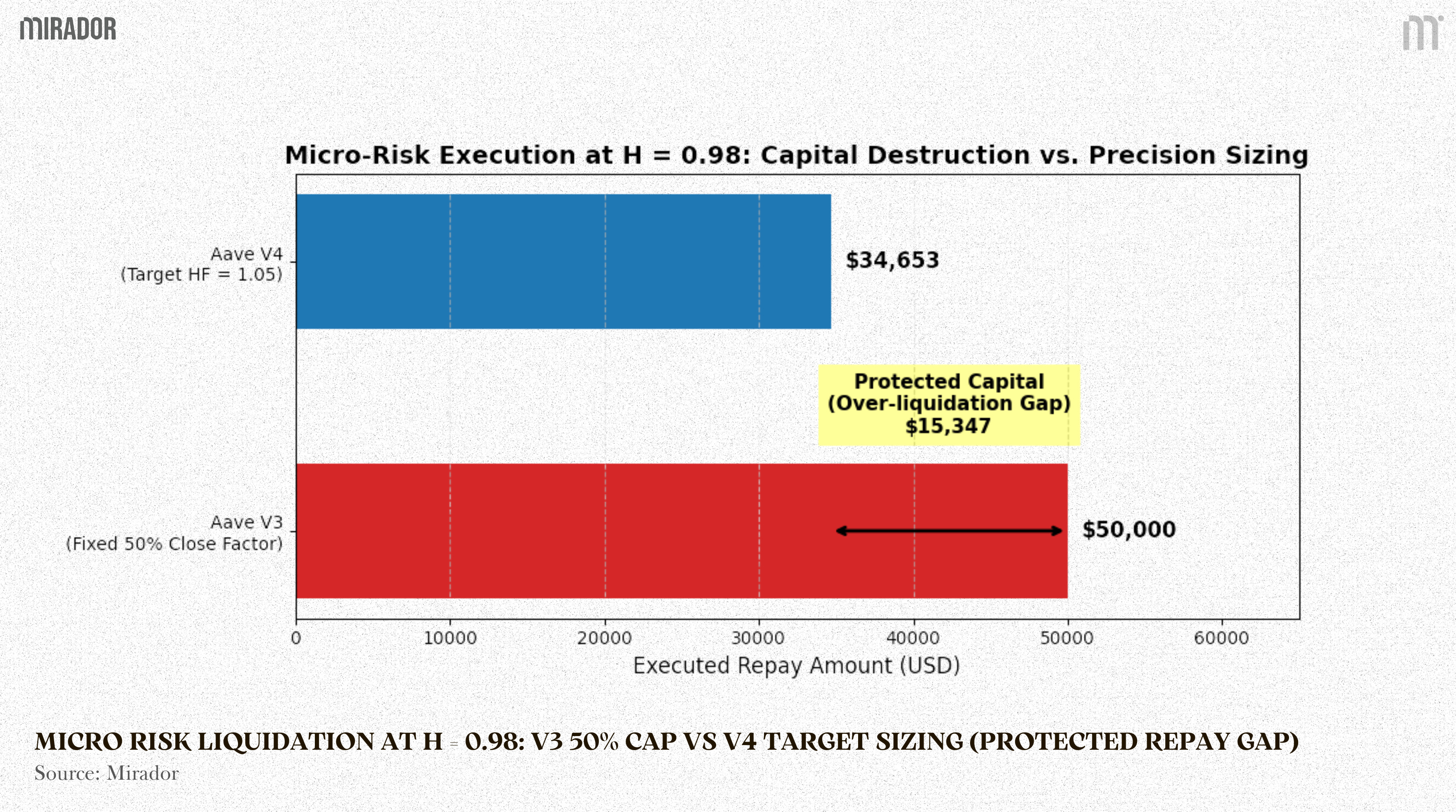
For this exact same position, the legacy V3 model allowed a maximum execution limit of 50 percent of the total debt (50,000 USD). Because liquidation bots are programmed to maximize absolute profit, they routinely submit executions right at this ceiling limit. The result is an artificially inflated Health Factor that destroys user capital.
By embedding control theory mathematics into the core Smart Contract, the _calculateDebtToTargetHealthFactor function in V4 caps the required intervention at 34,653 USD. This provides direct technical proof that V4 utilizes the absolute minimum force necessary to secure the system, completely eliminating the excess capital destruction zone inherent to the legacy model.
C/ VARIABLE BONUS AND LIQUIDATOR COMPETITION
When Target Health Factor sizing compresses the repay amount R(H) near the threshold, liquidators earn less absolute revenue per liquidation. Gas and execution costs do not shrink at the same rate. So the protocol needs a second lever to keep keepers participating, especially when positions are only slightly unsafe.
Aave V4 uses a state based Dutch auction mechanism to do this. There is no orderbook of bids. Instead, the protocol publishes a deterministic bonus schedule b(H). As the position becomes riskier and H falls, the bonus increases. The auction emerges implicitly because multiple keepers observe the same public schedule and choose when to execute based on their own cost structure.
If this is an auction, what is the clock? The market is the clock. H moves because collateral prices move and because debt grows over time from interest. That market driven drift acts like the auction tick. The reward increases until it reaches a keeper’s break even point.
1. The Piecewise Bonus Curve
The purpose of this subsection is to define the exact incentive schedule that keepers observe, because this schedule is the economic engine behind the state based Dutch auction. In the next steps, we will plug b_net(H) directly into the keeper profit function π_i(H) to derive the break even point (H^*)_i, the Dead Zone, and the Race Band.
The codebase manages the raw liquidation bonus b(H) via three parameters: the maximum bonus cap (b_max), the maximum risk threshold (H_max), and the minimum bonus (b_min).
Intuition first. The schedule has three regions:
· If 𝐻≥1.0, liquidation is not allowed, so the bonus is zero.
· If 𝐻_𝑚𝑎𝑥<𝐻<1.0, liquidation is allowed and the bonus increases linearly as 𝐻H deteriorates, starting from 𝑏_𝑚𝑖𝑛.
· If 𝐻≤𝐻_𝑚𝑎𝑥, risk is severe and the bonus is capped at 𝑏_𝑚𝑎𝑥.
Mathematically, b(H) is strictly defined as a piecewise function:
However, the actual bonus captured by the liquidator is discounted by the protocol fee (f_protocol). The net bonus function is locked by the following formula:
Near the threshold (𝐻≈1), the repay amount 𝑅(𝐻) produced by target sizing is small, so keeper revenue is highly sensitive to the bonus level. As 𝐻 deteriorates, 𝑏_𝑛𝑒𝑡(𝐻) increases, raising expected revenue until it becomes profitable for some keeper to execute. This is exactly the mechanism that creates a break even root 𝐻^* and explains why keepers may wait inside a Dead Zone instead of racing immediately at 𝐻<1.
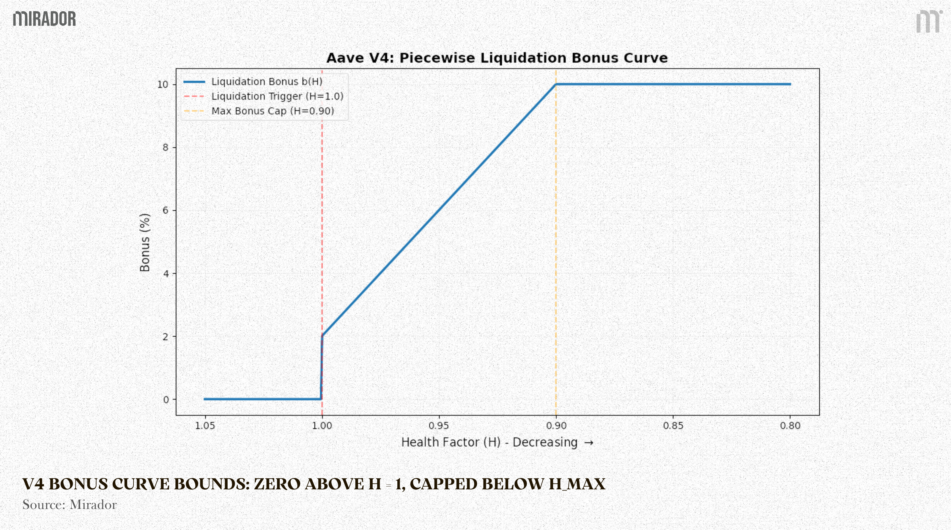
The mathematical bounds of the V4 piecewise liquidation bonus curve, illustrating zero incentive above H=1.0 and a strict cap below H_max.
2. The Profit Equation and the Break-even Root
A bot’s decision to execute the liquidateCall() function does not depend on the nominal bonus percentage, but is strictly governed by its net profit function π(H).
Given a target repay volume R(H), gas cost g_i, and DEX slippage cost s_i specific to bot i, the net profit equation is established as:
A bot will only execute a transaction when π_i(H)>0. The break-even point for bot i, denoted as (H^*)_i, is the exact root of the boundary equation:
3. The Dead Zone and the Waiting Game Logic
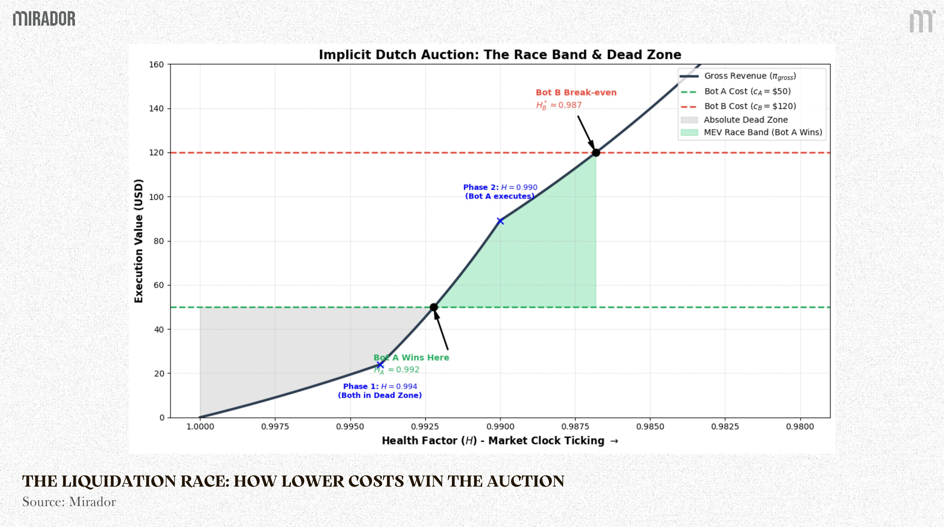
To observe how the implicit Dutch Auction dictates bot behavior, we must model the competition between multiple liquidator bots. The auction does not happen via an explicit orderbook. It is a race governed by execution costs.
Assume a macro position where the Target is 𝑇=1.05, total debt is 𝐷=5,000, and 𝜏=0.80.
We introduce two competing liquidator bots with distinct structural costs (𝑐_𝑖=𝑔_𝑖+𝑠_𝑖):
· Bot A (Optimized Searcher): Utilizes private RPCs and highly efficient routing. Total cost 𝑐_𝐴=50 USD
· Bot B (Standard Liquidator): Operates on public mempools with average slippage. Total cost 𝑐_𝐵=120 USD.
Phase 1: The Dead Zone (𝐻=0.994)
The market dips slightly. 𝐶=4,970 USD →𝐻=0.994
At this nominal risk level, the interpolated bonus is extremely low, e.g., 𝑏=0.02
Applying the Target HF sizing solver:
Gross profit is: 1,196.58×0.02=23.93 USD
Let us calculate the net profit 𝜋_𝑖(𝐻) for both bots:
System Result: Both 𝜋_(𝐴 )and 𝜋_𝐵 are strictly negative. The transaction falls into the Dead Zone. No bot is economically willing to execute. The market clock ticks, forcing the auction to wait.
Phase 2: The Auction Execution (𝐻=0.990)
The market drops further. 𝐶=4,950 →𝐻=0.990.
The risk deepens, scaling the interpolated bonus up to 𝑏=0.06.
Recalculating the execution size 𝑅:
Gross profit expands to: 1,485.15×0.06=89.11 USD.
Now, we observe the Dutch Auction resolution:
System Result: Bot A’s Expected Value turns positive. Bot A immediately signs and broadcasts the liquidateCall() transaction. The debt is dynamically repaid, and the position is restored to 𝐻=1.05.
Bot B never gets the chance to liquidate. Because Bot A has a superior cost structure, it mathematically wins the Dutch Auction by intervening at a higher 𝐻 (a shallower risk depth) where Bot B is still trapped in the Dead Zone. This mechanism forces liquidator bots to optimize infrastructure and routing efficiency, so the protocol can be secured earlier with less collateral seized than a late, deeper liquidation.
4. The Race Band and the MEV Shift
The core shift in V4 is not that MEV disappears. The shift is that the trigger for competition changes shape.
In Aave V3, the system is close to a single ignition point. Once 𝐻 crosses below 1.0, a fixed bonus can make Expected Value turn positive for many liquidators at the same boundary. That concentrates competition at one line, often creating Priority Gas Auctions.
In Aave V4, profitability is state dependent. Because 𝑅(𝐻) is compressed near the threshold and the bonus increases as 𝐻 deteriorates, Expected Value does not turn positive for everyone at once. Instead, it turns positive first for the most cost efficient liquidator bots.
Each bot has different optimization capabilities for gas (𝑔_𝑖) and slippage (𝑠_𝑖). Their absolute execution cost is:
In this implicit auction, a bot effectively bids through its cost structure by signaling: I will execute as soon as the public reward covers my private cost. A bot with better routing or private orderflow has a lower 𝑐_𝑖, so it can execute earlier at a higher health factor where the bonus is still lower, but profit is already positive for that bot.
This is what creates the Race Band.
Mechanism definition: The Race Band is the range of 𝐻H where the most optimized tier of bots transitions from 𝜋(𝐻)<0 to 𝜋(𝐻)>0. In other words, it is the golden window where Expected Value becomes positive for top tier bots, but is still negative for the rest.
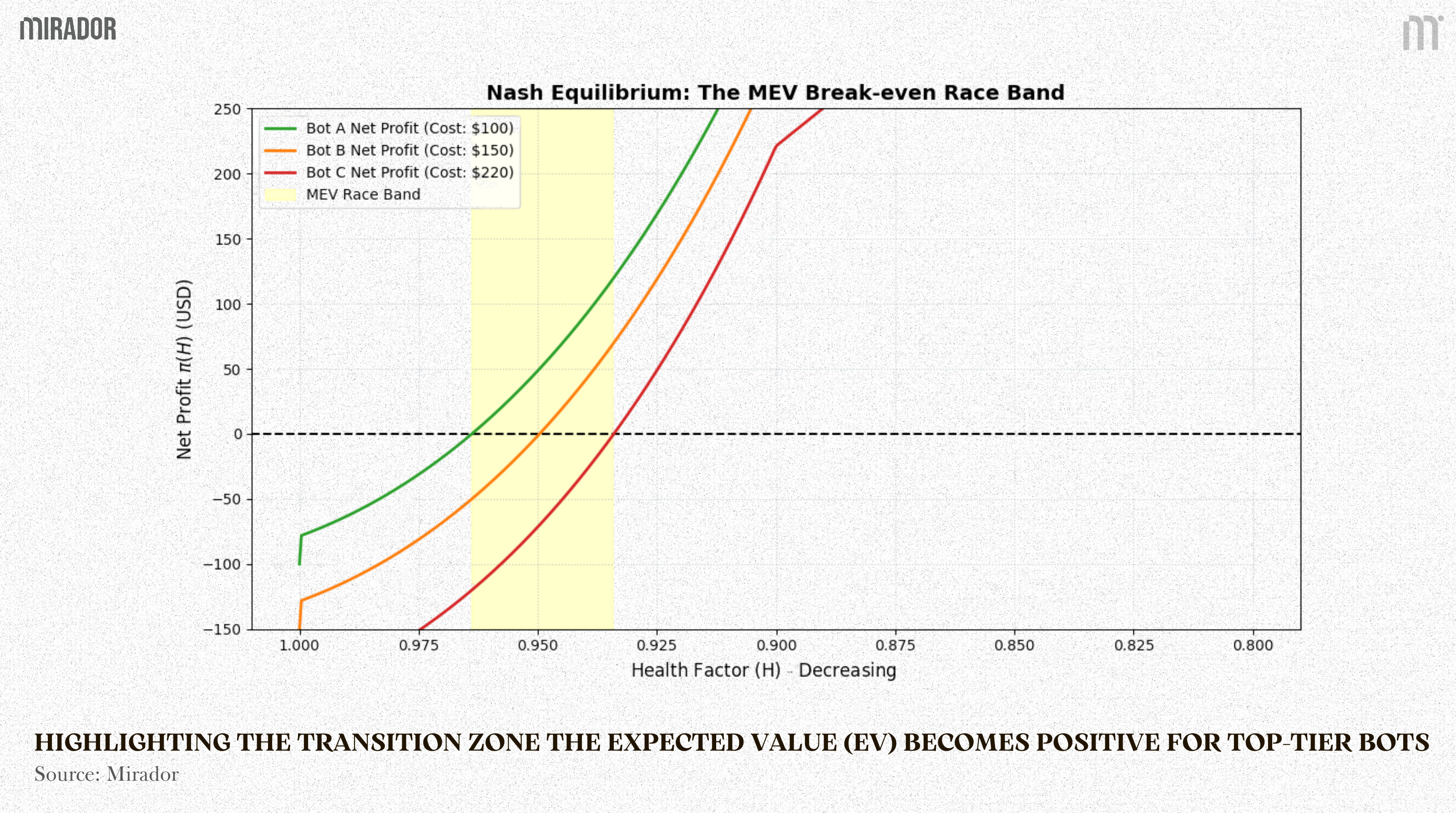
System Conclusion: Aave V4 does not eliminate MEV or Priority Gas Auctions (PGA). It merely shifts the ignition point from a static legal boundary (H=1,0) to a dynamic economic band (H≈(H^*)_i). Once market conditions push a position into the Race Band, the Expected Value (EV) turns positive, and actors will immediately burn Gas to secure execution rights. Consequently, the protocol minimizes the seized collateral volume while forcing Keepers to compete aggressively on structural cost efficiency, rather than engaging in the blind speed-racing inherent to V3.
CONCLUSION
Through rigorous source code dissection and on-chain empirical simulation, Aave V4 demonstrates a fundamental architectural shift: the transition from static legal constants to dynamic mathematical control functions.
By embedding the Target Health Factor into the execution sizing core and interpolating the liquidation bonus via a state-based auction mechanism, the V4 architecture definitively resolves two core DeFi paradoxes:
Capital Efficiency: It completely eliminates the capital destruction zone inherent to the V3 50% Close Factor’s over-liquidation logic. This maximizes user asset protection, preventing excessive capital seizure during micro-violations.
System Solvency: It restructures the game theory of the Keeper network. V4 shifts the MEV ignition point into a converging break-even Race Band, ensuring that toxic debt is reliably cleared by bots possessing the most optimized cost structures, requiring only the absolute minimum systemic intervention.
In Aave V4, liquidation is no longer a blind, punitive asset seizure. It has evolved into a quantitative self-rebalancing mechanism, mathematically secured and precise down to the wei.
DISCLAIMER
In this article, we focus on Aave V4 liquidation mechanics, specifically Target Health Factor repay sizing and the state based liquidation bonus curve. Rather than evaluating overall protocol performance or making broad claims that one design is always superior, our goal is to break down the core design logic and execution mechanics that shape borrower outcomes and liquidator incentives.
We do not avoid technical details. The article includes smart contract flow, mathematical formulas, and simplified game theory. However, all models, examples, and calculations are intentionally simplified and explained step by step to make the mechanisms clear and intuitive for readers with different levels of DeFi experience. Where we use empirical charts derived from Aave V3 on chain data, the results should be read as evidence of patterns under specific assumptions, not as universal guarantees.
Ahead of the Aave V4 launch, we will return with additional deep dives on other parts of the architecture, including risk parameter design choices, incentive tradeoffs, and edge cases under market stress.