

YIELD BASIS LEVAMM - PART I: THE ALGORITHM
Breaking down the algorithm behind Yield Basis’s leverage rebalancing mechanism

If you found this useful, the full breakdown with math and simulation is on Substack → [mirador.finance] More deep-dives incoming.
Join our Telegram to get notified first → [https://t.me/Miradortelegram]
INTRODUCTION
Yield Basis BTC/crvUSD pools have been far away from the ideal 50/50 BTC–crvUSD balance, which causes TRD rise and puts pressure on the crvUSD peg.
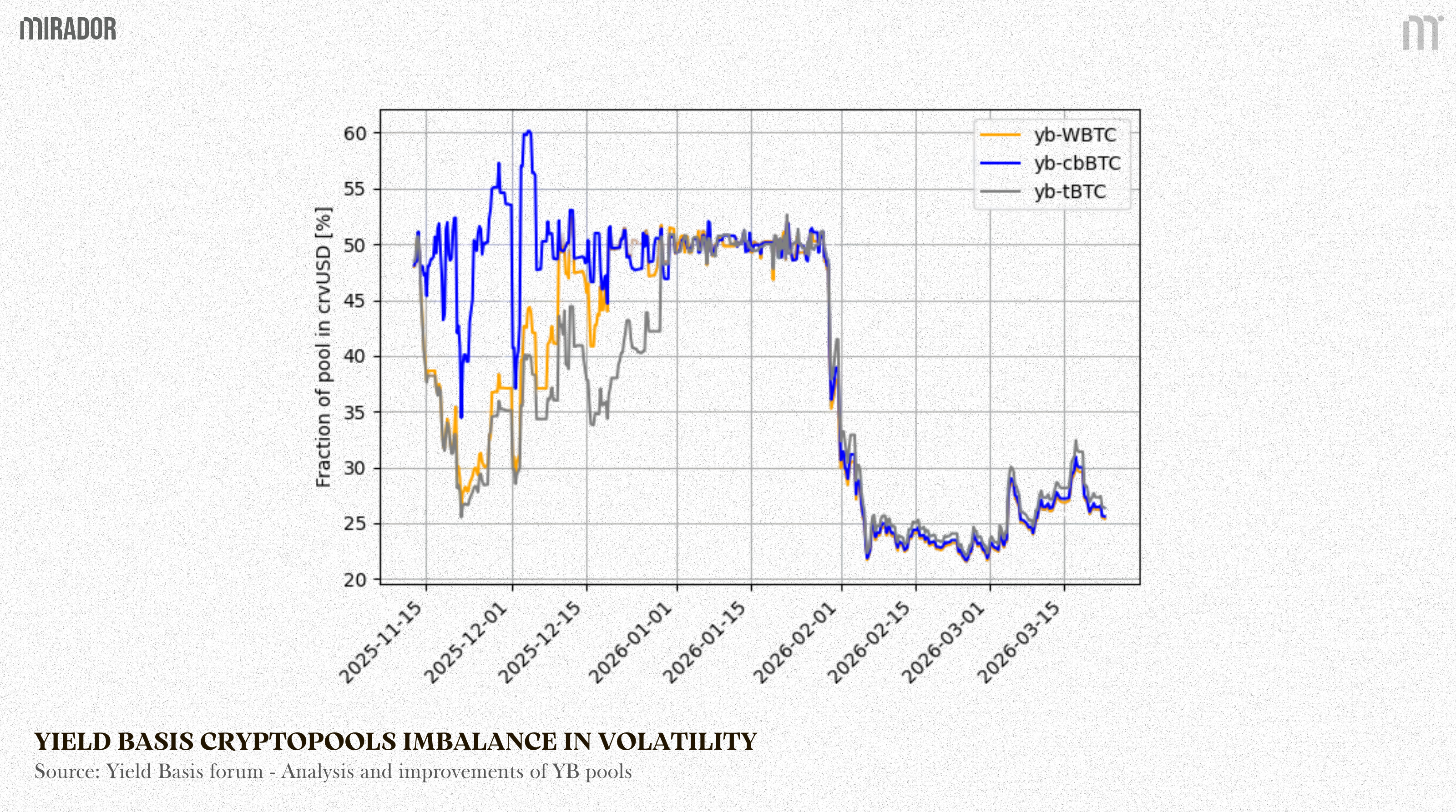
Source: Yield Basis forum - Analysis and improvements of YB pools
In Part 1, we break down the core mechanics of LEVAMM: how the pool is designed to maintain the theoretical 50:50 balance. This is the foundation of Part 2, which discusses how this connects to the other components of the system, including the Cryptoswap pool and the virtual pool in practice.
KEY TAKEAWAYS
The core objective of Yield Basis is to enable liquidity provision without impermanent loss. This is achieved by maintaining each liquidity position at a constant leverage level of L=2.
However, when the asset price changes, the leverage ratio deviates from this target. The LEVAMM contract is designed to handle this adjustment: it functions as a specialized AMM that automatically re-leverages the position through arbitrage, restoring the intended leverage level.
A static AMM curve cannot keep leverage constant when price changes.
To maintain constant leverage, the bonding curve itself must depend on the oracle price p0.
For each p0, LEVAMM defines one unique curve and one unique equilibrium point.
For every price level, there is only one equilibrium point engineered so that the position returns to the 2x leverage.
Writer’s note:
LEVAMM is difficult to explain without some math, because its core logic comes from how the invariant changes with the oracle price and how that brings the system back to its target leverage. For that reason, this article is intentionally detailed, but easy to follow step by step.
If some parts feel dense at first, we’d encourage you to go through them patiently and in order, since each section builds directly on the previous one.
SECTION 1: AUTO LEVERAGE AMM (LEVAMM) IN YIELD BASIS FLOW
In the previous article, we have disscussed that: The core objective of Yield Basis is to enable liquidity provision without impermanent loss. This is achieved by maintaining each liquidity position at a constant leverage level of L=2.

However, maintaining a 2x leveraged position through manual re-leveraging is inefficient, costly, and structurally imprecise. That is exactly why Yield Basis expresses the user’s position through AMM functions, so that:
Rebalancing is triggered automatically by creating arbitrage opportunities through the AMM curve.
The cost of executing rebalancing is shifted from the user to arbitrageurs, who are incentivized to perform the trade in order to capture the price spread.
What’s in LEVAMM?
When a user deposits WBTC, the protocol adds matching crvUSD from its credit line and supplies both into the Curve WBTC/crvUSD pool. In return, Curve mints LP tokens, and those LP tokens are held by the LEVAMM.
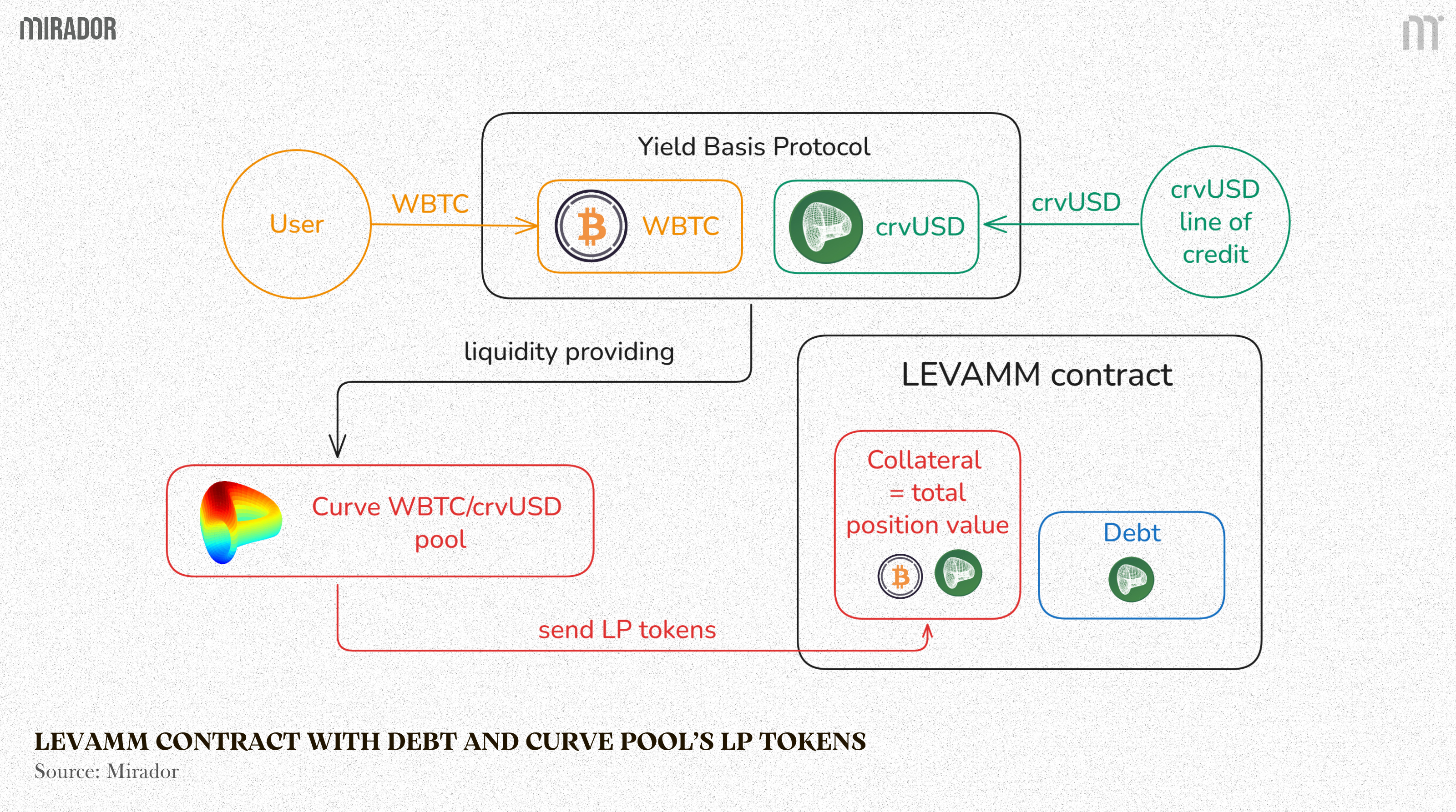
In this setup, the LP tokens from Curve pools are treated as the collateral because it represents the total position value inside the pool. The debt is the amount of crvUSD the protocol borrowed to build that position. In a LEVAMM, we have:
Collateral (y): the Curve LP position, representing the full WBTC + crvUSD pool exposure
Debt (d): the borrowed crvUSD used to create that LP position
The idea of Yield Basis is to model the relationship between d and y in a way that is similar to the relationship between x and y in a traditional AMM.
Invariant idea: solving the problems
The idea of creating an AMM for d and y, however, immediately raises some problems.
(1) A standard AMM can automate trading, but it cannot keep leverage fixed.
As we showed in Part 2 of article series “IMPERMANENT LOSS AND HOW Yield Basis MAKES IT ‘ZERO’”, any AMM that operates by moving along a curve will naturally cause leverage to change over time. That is also the source of impermanent loss for LPs.
In other words, a standard curve-based AMM can automate trading, but it cannot keep leverage fixed.
This is the core challenge Yield Basis is trying to solve:
Using the automatic market-making and rebalancing power of an invariant
At the same time, using that mechanism to maintain a constant 2x leveraged position
A standard AMM cannot do both on its own.
(2) Yield Basis rebalancing requirement: debt and collateral move in the same direction
Under normal conditions, position’s leverage level naturally drifts when prices move. To keep leverage fixed at a target level 2x to eliminate impermanent loss, in essence, a Yield Basis position is continuously adjusted by either repaying or borrowing additional crvUSD, for example:
When WBTC price increases (leverage falls below the target), it borrows more crvUSD;
When WBTC price decreases (leverage rises above the target), it repays crvUSD debt.
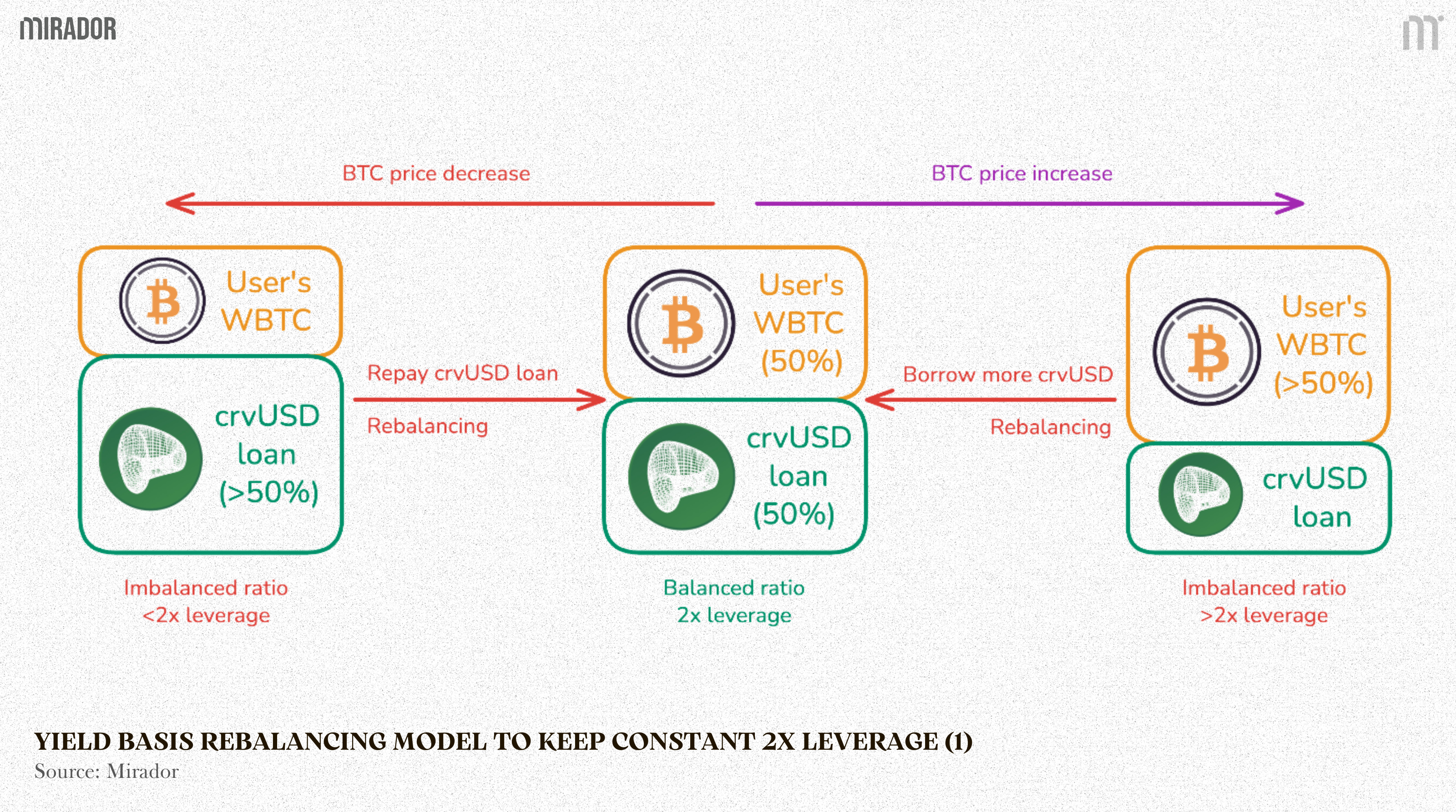
In other words, the collateral value (WBTC) and the debt amount (crvUSD) must move in the same direction.
However, a normal AMM with two reserves (x,y), using the usual AMM formulas:
always creates an offsetting relationship between the two state variables: when x increases, y decreases.
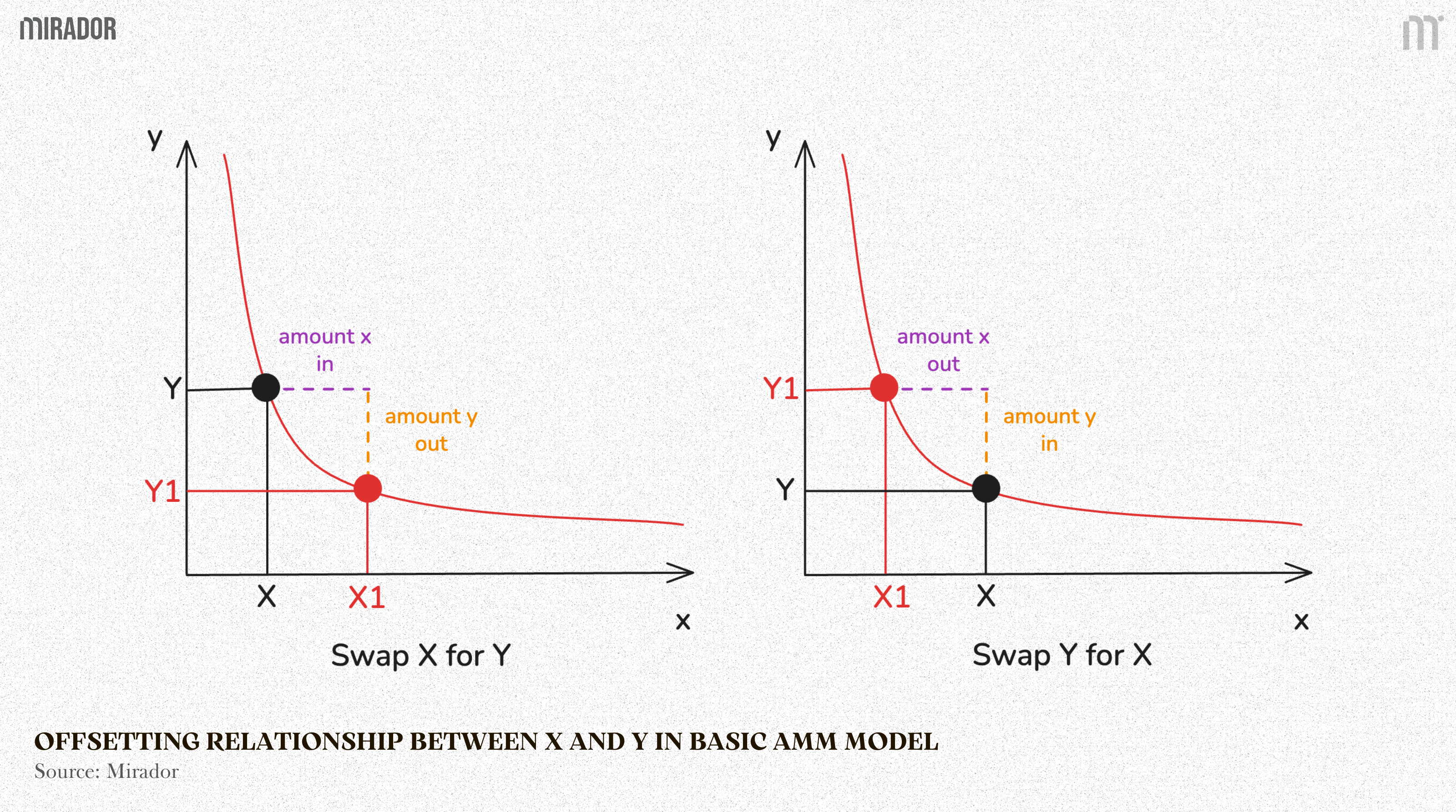
This offsetting runs against what Yield Basis wants to achieve.
To solve these 2 problems, Yield Basis changes the internal structure of the AMM itself. In particular, it introduces three major design changes.
To make debt (d) and y (collateral) move together, the system modifies the stablecoin reserve through a transformed variable, rather than use d directly.
To keep 2x leverage in every market price, they brings in p0, (the real-time oracle price of the volatile asset, such as WBTC).
As a result, instead of using one single static curve, Yield Basis uses p0 to define different curve for each market price.
These three ideas are the core of the design. In the next sections, we will examine each of them in detail.
SECTION 2: LEVAMM INVARIANT
1/ LEVAMM with virtual stablecoin reserve
To create required rebalacing effect, the system does not expose the debt variable d (debt in crvUSD) directly to the AMM function. Instead, it defines a new state variable,
with:
x0 is virtual stablecoin reserve (a function determined by the external reference price p0); Yield Basis relies on an external BTC/USD oracle and effectively assumes that crvUSD always stays at 1 USD. That makes the model cleaner, but it also creates an obvious risk: if crvUSD depegs, the pool may no longer be pricing things correctly.
We will come back to this in Part 2.
d is the current stablecoin debt; as debt gets close to x0, borrowing one more small unit of x requires a disproportionately large amount of y. In other words, slippage becomes extreme near the boundary.
With this redefined reserve, the LEVAMM no longer operates on the raw debt variable d, but on the virtual reserve x = x0 − d. The invariant therefore becomes:
where d is the debt, y is the amount of collateral and invariant I is constant at the a specific market price (po).
Assume at a specific p0, I=100 000, then the pool follows the invariant:
In practice, finding x0 for each price p0 takes a few calculation steps, which we will explain below. For now, to keep the example simple, we just assume x0=15 000 as a precomputed value.
The rule is simple: no matter what happens, this product must always stay equal to 100000.
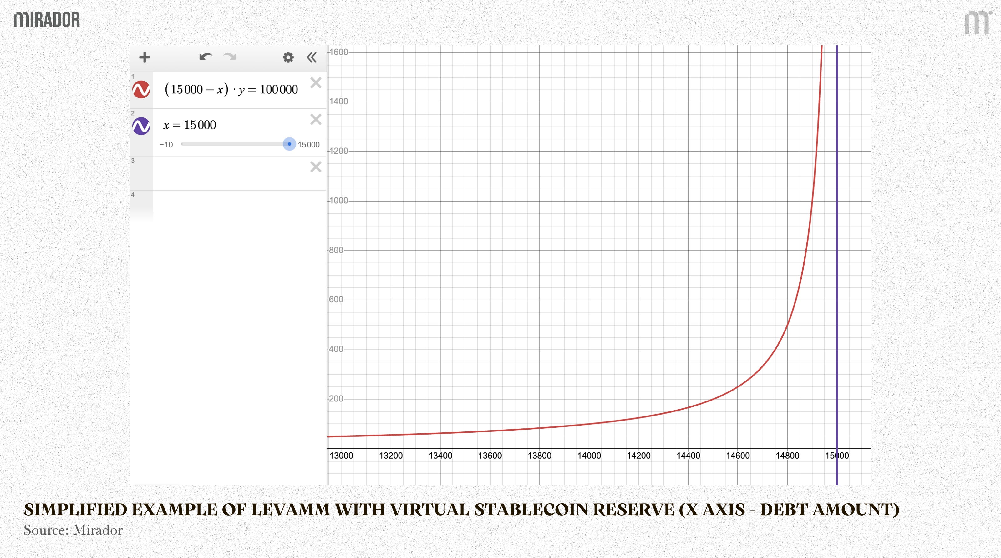
Unlike a standard Uniswap curve, this curve slopes upward from left to right. That upward shape reflects the key property of the invariant: debt and collateral move in the same direction. In this graph, the horizontal axis is labeled x (but here x is standing in for debt because of the platform’s notation).
So as d increases, y also increases, and vice versa, which is exactly the co-movement Yield Basis wants.
The charst below shows the AMM view, both present x*y=k model, while the left one is Yield Basis’ curve where x (or u in the chart) = x0 − d. That means u and collateral y move in opposite directions, just like a normal AMM.
Besides, the right chart shows the same structure rewritten in terms of debt d. Since d = x0 − u, the inverse relation is flipped, so d and y now move in the same direction.
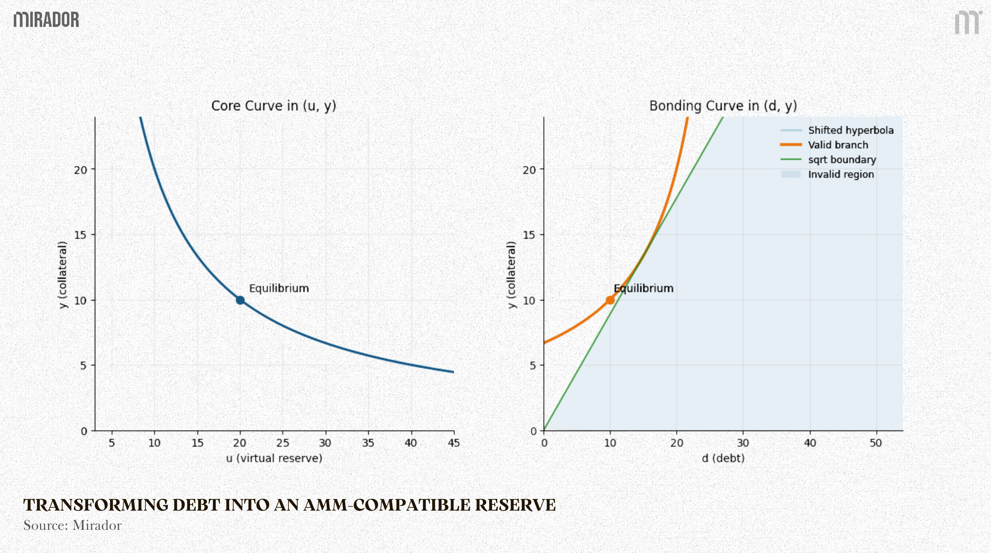
This is exactly the point of the design: it keeps debt and collateral positively aligned at the position level, while still preserving the automatic pricing and rebalancing benefits of a constant-product AMM.
LEVAMM does not create impermanent loss in the usual spot-AMM sense, because it is not simply rebalancing a passive two-asset inventory. Instead, it rebalances a leveraged position by allowing arbitrage to reduce debt and restore the target leverage.
2/ Different invariants and balance points for different market prices
In a static AMM with the invariant x.y=k, when the market price changes, the equilibrium point moves along the fixed curve.
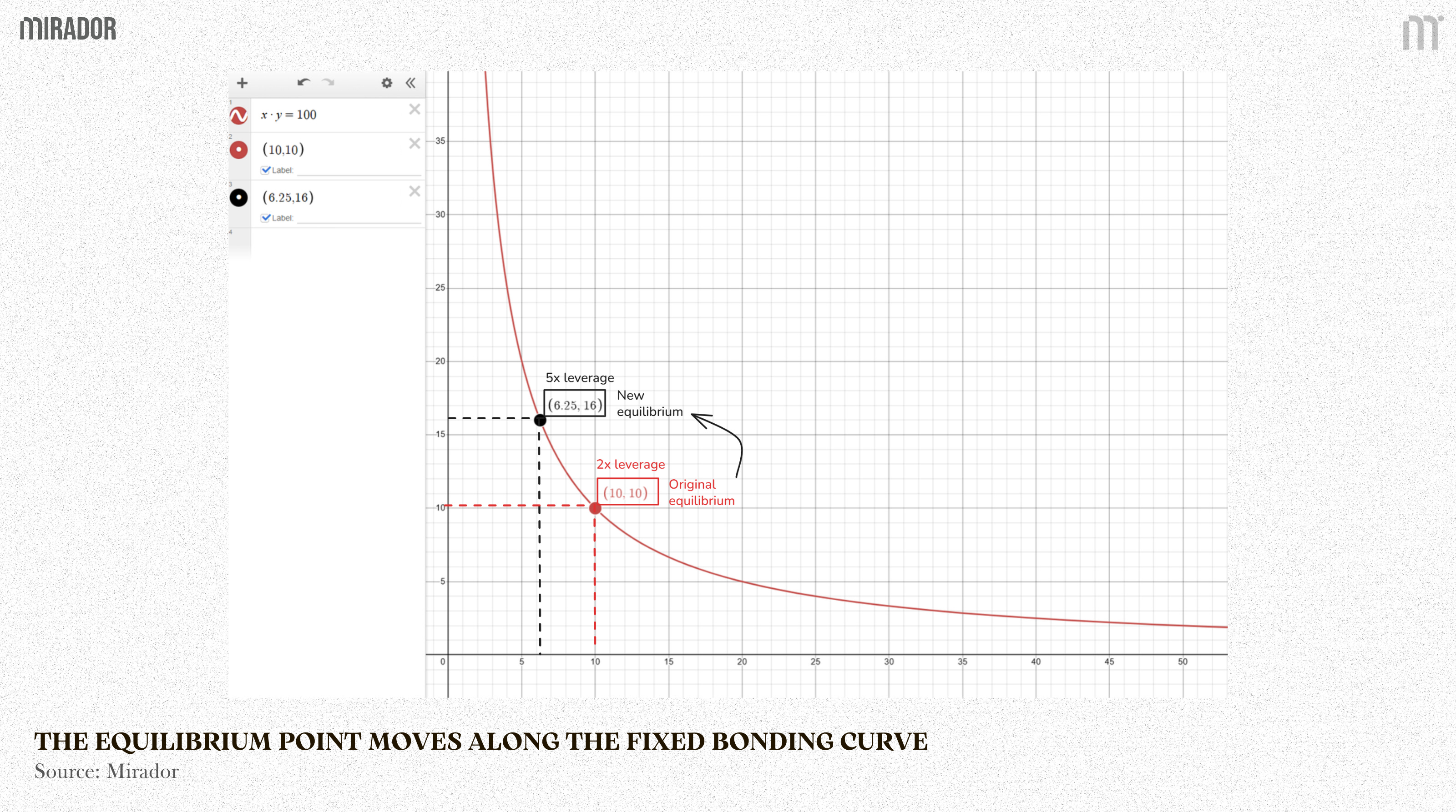
The equilibrium point moves along the fixed bonding curve (Source: Desmos – Mirador)
The issue is that this curve does not preserve leverage.
The chart shows how a leveraged LP position moves along a fixed x*y=100 curve when price changes.
It starts at (10,10) with 2x leverage. After price falls, the pool rebalances to (6.25;16). Even though the position is now worth less, the debt remains unchanged. That causes equity to shrink and leverage to jump to 5x.
Important note: This is a deliberately simplified example, used only to show the core idea as clearly as possible.
In other words, the problem is that a fixed AMM causes leverage to drift away from its target whenever market price changes.
Therefore, LEVAMM is designed to solve this by adjusting the curve at each market price. For every price level, there is only one equilibrium point engineered so that the position returns to the desired leverage, here is 2x.
(1) Equilibrium point at each specific market price
Yield Basis adjusts the curve for each market price so that the new equilibrium satisfies that debt condition.
Unlike a static AMM, the curve is no longer fixed once and for all. x0 (virtual stablecoin reserve) is defined as a function depends on the oracle price p0.
Therefore, the invariant term I also becomes a function of p0. This price-dependent design is reflected directly in the final LEVAMM invariant:
As a result, in LEVAMM, the curve itself is redefined at each price level. As p0 changes, the parameters of the curve change with it, each price has its own bonding curve and equilibrium.
In other words, at every oracle price, there is one unique equilibrium where the position returns to exactly 2x leverage.
(2) Defining x0(p0) function
The idea of defining x0 as a function of p0 is simple: each market price p0 should have its own bonding curve, and the equilibrium on that curve should be the one that gives exactly 2× leverage.
Once this is set up, we can start by defining x0 at the equilibrium point itself (p = p0)
Step 1: Finding x0 at p = p0
For any oracle price p0, there is an ideal debt level that is consistent with the target leverage L:
In the 2x case, this simplifies to:
In a basic AMM such as Uniswap v2, the price p at any point on the curve is given by the ratio of the two reserves:
Therefore, when p = p0, the pricing formula of the pool becomes:
Replace , we have
then
Therefore, for fixed , x0 is a function of p0 following that .


However, swaps can move the pool’s price away from real market price.
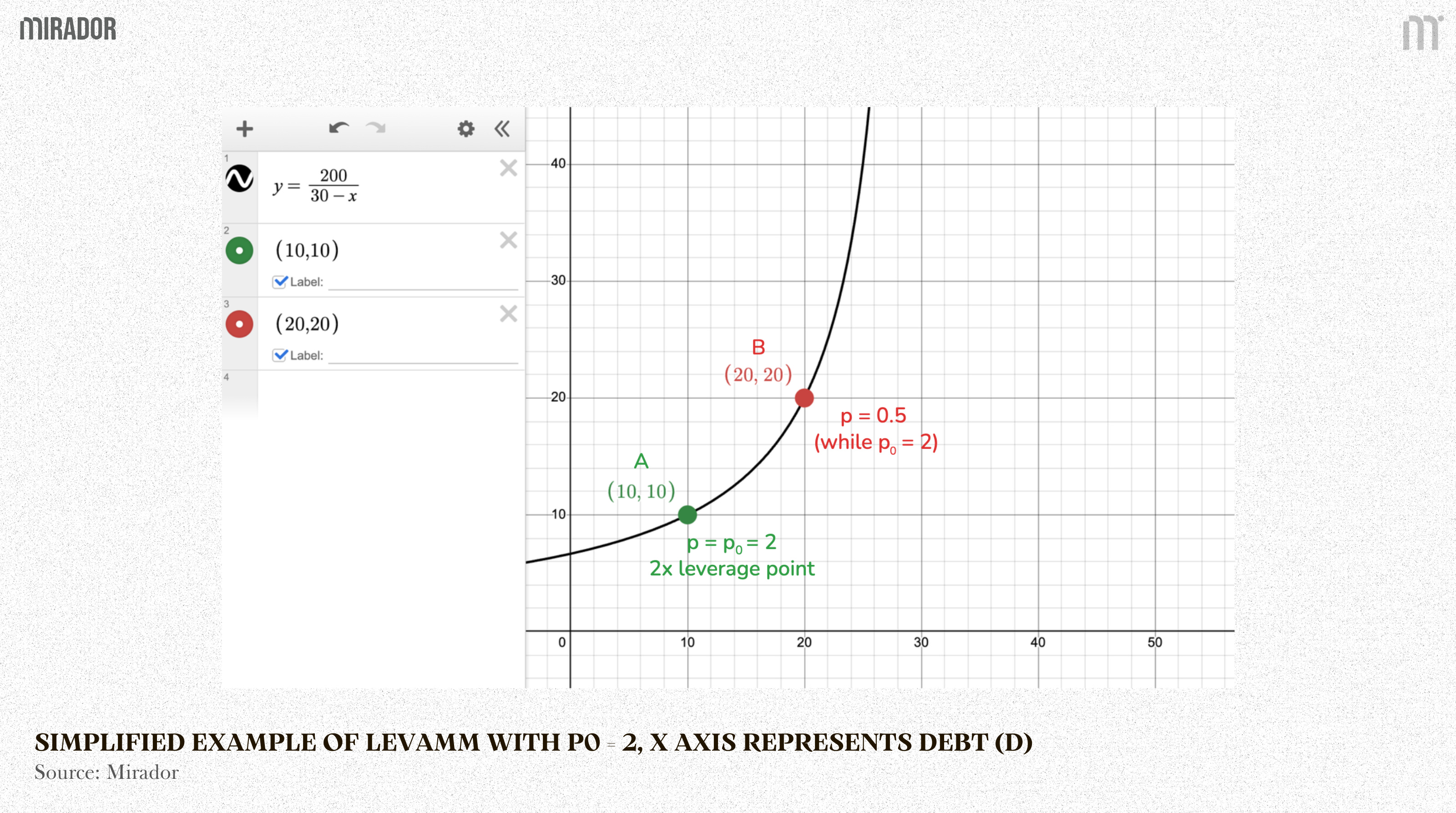
For example, assume the oracle price is p0 = 2. LEVAMM is designed so that, for this specific price level, the bonding curve is:
(this is a highly simplified invariant, included only for illustrative purposes)
This bonding curve’s equilibrium is A=(10,10), where the internal pool price matches the oracle price, p = p0 = 2, and the position maintains the desired leverage of 2x.
Even at a fixed oracle price, the pool does not always remain exactly at the oracle-aligned equilibrium. Normal user swaps can temporarily push the pool away from that point, so the internal pool price may deviate from the oracle price (for example: from A to B) until arbitrage activities brings it back.
So the goal now is to find a general function of x0 such that arbitrage on the curve naturally brings the pool back to that equilibrium of 2× leverage.
Step 2: Building invariant for every y, d at a specific p0
As the principle of AMM, at a market price, the invariant I in the actual state must still be equal to the invariant I in the ideal state, so that:
With
Y(x0-d) is I in actual state
- \(y(x_0 - d) = \tilde{y} \left( x_0 - \frac{p_0 \tilde{y}}{2} \right)\)
is I in ideal state (calculated in the previous step)
Or
After basic transformation, we have:
Solving for x0 and taking the larger root gives:
Finally, substituting this expression for x0 (p0) back into the invariant, we obtain the specific bonding curve associated with the oracle price p0, we get:
This means that once the oracle price p0 is fixed, the solved expression for x0 (p0) fully determines the bonding curve. So the invariant is no longer abstract: it becomes the specific curve that governs pool states at that oracle price.
(3) The final flow
Now, let’s connect all these things we have discussed before to see how LEVAMM interact with market changes
Step 1: Balanced state
Suppose the first state of YB WBTC/crvUSD pool is:
Oracle price: 70,000 crvUSD for 1 LP token (for example: LP token of WBTC/crvUSD pool).
Collateral amount (y): 10
Total Collateral Value = 700,000 crvUSD
Debt: 350,000 crvUSD.
The current leverage is:
So the position is perfectly balanced.
Step 2: Market price (oracle price p0) changes
Now suppose the oracle price drops from 70,000 to 63,000.
This is a large one-step move, so the resulting adjustment is also visually large. That makes it easier to show how the invariant determines x0 and the virtual LEVAMM state, how the AMM creates an arbitrage incentive, and how arbitrage flow pushes the position back toward the target leverage.
In practice, the mechanism does not need to wait for a large price drop like the one in this example.
The position becomes:
New oracle price (po): 63,000
New collateral value: 10×63,000=630,000
Debt remains: 350,000 crvUSD
The new leverage is:
The leverage is now above the target of 2.0. At this point, LEVAMM activates.
Step 3: Recreate a new LEVAMM invariant from current state
The pool now needs to compute x0 to define its internal pricing curve for new oracle price
With our new state:
we have:
With x0 = 787,500, LEVAMM constructs a virtual constant-product AMM:
Its virtual reserves are:
Y reserve (collateral): Y = 10 LP token
X reserve (stablecoin): X = x0 − d = 787,500 − 350,000 = 437,500
So:
Now check the AMM’s internal price:
So the AMM is pricing a LP token at 43,750 crvUSD.
This is the key point:
External market price: 63,000 crvUSD per LP token
Internal AMM price: 43,750 crvUSD per LP token
So the system is intentionally underpricing LP token in order to attract arbitrage.
This unusually large price gap in this example is mainly a consequence of our intentionally extreme price assumption.
In practice, this gap rarely exists.
Step 4: Arbitrage
Arbitrage bots see a clear opportunity: buy LP cheaply from the pool and sell it externally at the higher market price.
Bots will trade (adding stablecoin into the pool and removing LP) until the AMM price rises from 43,750 to 63,000, matching the market price, using constant-product AMM math:
Substitute the numbers:
Step 5: New balanced state for new market price
So after arbitrage, the AMM moves to:
which means arbitrage bots added 87,500 crvUSD to the pool to receive 1.666667 LP.
This added crvUSD amount is used to repay debt, so the new debt becomes: 350,000 − 87,500 = 262,500 crvUSD.
Now calculate leverage again:
As you can see, the position has returned exactly to the target 2x leverage.
By solving the quadratic equation for x0, the system can determine exactly how much to underprice the collateral inside the AMM. That deliberate mispricing creates an opportunity for arbitragers, who then bring in precisely the amount of stablecoin needed to reduce debt and restore the target leverage.
SECTION 3: VIRTUAL POOL FOR ARBITRAGE
As we mentioned in Section 2, the system adjusts LP token’s internal price to create an arbitrage opportunity and thereby incentivize external rebalancing.
However, arbitragers, who play the key role to keep 2x leverage through LEVAMM, typically want to trade actual cryptocurrencies (for example: WBTC) for stablecoins, not LP tokens.
To bridge this gap, the system introduces a “virtual pool” smart contract. This contract coordinates the leverage AMM, the crypto pool, and crvUSD flash loans so that arbitrageurs can effectively swap real crypto (BTC) and stablecoins (crvUSD), while the protocol handles the LP token mechanics behind the scenes.
To make this clearer, we will analyze the flow in the case where the position is unbalanced when the collateral ratio is higher than the outstanding crvUSD debt. In this scenario, the arbitrage progress performs an exchange from the crypto asset to stablecoin within the virtual pool.
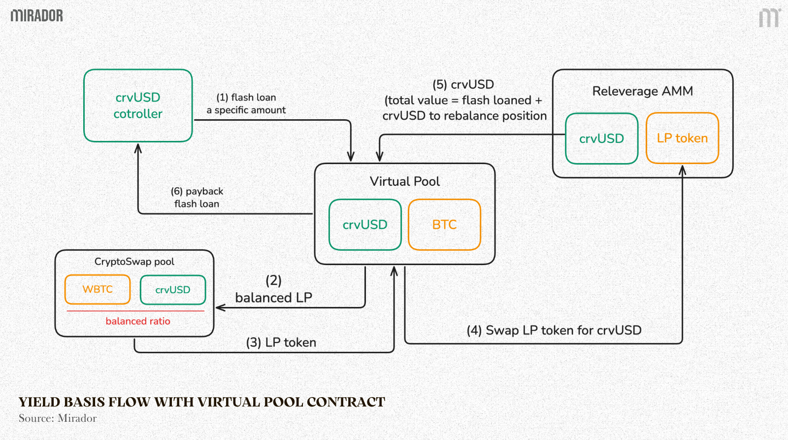
(1) Flash loan crvUSD (formula to calculate exact amount will be discussed below)
The system first takes a flash loan of crvUSD from the crvUSD controller. This amount is calculated precisely so it can be paired with the crypto asset to form balanced liquidity.
(2) Add balanced liquidity to the CryptoSwap pool
The borrowed crvUSD is combined with the crypto asset (e.g. WBTC) and deposited into the CryptoSwap pool at the pool’s current ratio. Because liquidity is added in the correct proportion, this action does not move the spot price in the pool.
(3) Receive LP tokens
After adding liquidity, the system receives LP tokens, which represent ownership of the balanced position in the CryptoSwap pool.
(4) Swap LP tokens for crvUSD in the Releverage AMM
These LP tokens are then sent to the Releverage AMM, where they are exchanged for crvUSD. Conceptually, this step converts collateral (LP tokens) into stablecoin debt through the AMM’s invariant.
(5) Collect crvUSD from the Releverage AMM
The Releverage AMM returns crvUSD. The total crvUSD received is enough to both: Repay the flash loan, and rebalance the user’s leveraged position as intended.
(6) Repay the flash loan
Finally, part of the crvUSD obtained from the Releverage AMM is used to repay the flash loan within the same transaction.
The opposite direction (exchanging from stablecoin to the crypto asset) follows the same logic and can be understood in an similar way.
The next question is: How do we calculate the exact amount of crvUSD that needs to be borrowed so the rebalance works out perfectly?
This value is determined by the following formula (more detail breakdown comes in part 2):
With φ is the needed amount of crvUSD to flashloan, we have other components:
1/ The user’s current position
d: existing debt
y: amount of collateral held in the leverage AMM
x0: known internal balance related to the position
2/ The state of the underlying CryptoSwap pool
xc, yc: total stablecoin and crypto liquidity in the pool
Sc: total LP token supply
These values determine how much stablecoin value each LP token represents.
3/ AMM execution costs
f: the leverage AMM fee, which is explicitly accounted for in the calculation.
This formula is used to calculate the exact amount of crvUSD that needs to be flash-borrowed so a rebalance can be completed perfectly in one transaction (φ)
The reason it takes the form of a quadratic equation is that solving this equation gives one correct value for the flash loan:
Borrow too little, and the rebalance cannot be completed
Borrow too much, and the flash loan cannot be fully repaid
The quadratic formula finds the exact middle point where everything balances: the position is rebalanced, fees are covered, prices are not disturbed, and the flash loan is repaid in full.
In Part 2 of this article, we will break down the interaction between the CryptoSwap AMM, LEVAMM, and the virtual pool, and examine how their interplay shapes the pricing of tokens within the pool.
CONCLUSION
The core innovation of Yield Basis lies in its ability to support liquidity provision without impermanent loss by maintaining each liquidity position at a constant leverage ratio of L = 2. Because changes in the asset price naturally push the position away from this target, a conventional static AMM curve is not enough. Preserving constant leverage requires the bonding curve itself to vary with the oracle price p0.
LEVAMM is designed precisely for this purpose. For every oracle price, it defines a unique invariant curve and a unique equilibrium point such that the position is restored to the target 2x leverage. This makes LEVAMM a specialized AMM whose role extends beyond pricing trades: it acts as an automatic re-leveraging engine. Through arbitrage, the system continuously rebalances the position back toward its intended state as market conditions evolve.
In short, Yield Basis replaces the static AMM paradigm with a price-dependent invariant tailored to leverage stability. The result is a mechanism that preserves the self-correcting properties of AMMs while engineering a single valid equilibrium at every price level, ensuring that liquidity positions remain aligned with the protocol’s no-impermanent-loss design goal.
Should emphasis the price 63000 is the LP price not the BTC price offered by the AMM pool.